Download
1 / 49
520 likes | 794 Views
Scale-Invariant Feature Transform (SIFT). Jinxiang Chai. Review. Image Processing - Median filtering - Bilateral filtering - Edge detection - Corner detection. Review: Corner Detection. 1. Compute image gradients

E N D
Scale-Invariant Feature Transform (SIFT) Jinxiang Chai
Review Image Processing -Median filtering - Bilateral filtering - Edge detection - Corner detection
Review: Corner Detection 1. Compute image gradients 2. Construct the matrix from it and its neighborhood values 3. Determine the 2 eigenvalues λ(i.j)= [λ1, λ2]. 4. If both λ1 and λ2 are big, we have a corner
The Orientation Field Corners are detected where both λ1 and λ2 are big
Good Image Features • What are we looking for? • Strong features • Invariant to changes (affine and perspective/occlusion) • Solve the problem of correspondence • Locate an object in multiple images (i.e. in video) • Track the path of the object, infer 3D structures, object and camera movement,
Scale Invariant Feature Transform (SIFT) • Choosing features that are invariant to image scaling and rotation • Also, partially invariant to changes in illumination and 3D camera viewpoint
Invariance • Illumination • Scale • Rotation • Affine
Required Readings • Object recognition from local scale-invariant features [pdf link], ICCV 09 • David G. Lowe, "Distinctive image features from scale-invariant keypoints,"International Journal of Computer Vision, 60, 2 (2004), pp. 91-110
Motivation for SIFT • Earlier Methods • Harris corner detector • Sensitive to changes in image scale • Finds locations in image with large gradients in two directions • No method was fully affine invariant • Although the SIFT approach is not fully invariant it allows for considerable affine change • SIFT also allows for changes in 3D viewpoint
SIFT Algorithm Overview • Scale-space extrema detection • Keypoint localization • Orientation Assignment • Generation of keypoint descriptors.
Scale Space • Different scales are appropriate for describing different objects in the image, and we may not know the correct scale/size ahead of time.
Scale space (Cont.) • Looking for features (locations) that are stable (invariant) across all possible scale changes • use a continuous function of scale (scale space) • Which scale-space kernel will we use? • The Gaussian Function
Scale-Space of Image • variable-scale Gaussian • input image
Scale-Space of Image • variable-scale Gaussian • input image • To detect stable keypoint locations, find the scale-space extrema in difference-of-Gaussian function
Scale-Space of Image • variable-scale Gaussian • input image • To detect stable keypoint locations, find the scale-space extrema in difference-of-Gaussian function
Scale-Space of Image • variable-scale Gaussian • input image • To detect stable keypoint locations, find the scale-space extrema in difference-of-Gaussian function Look familiar?
Scale-Space of Image • variable-scale Gaussian • input image • To detect stable keypoint locations, find the scale-space extrema in difference-of-Gaussian function Look familiar? -bandpass filter!
Difference of Gaussian • A = Convolve image with vertical and horizontal 1D Gaussians, σ=sqrt(2) • B = Convolve A with vertical and horizontal 1D Gaussians, σ=sqrt(2) • DOG (Difference of Gaussian) = A – B • So how to deal with different scales?
Difference of Gaussian • A = Convolve image with vertical and horizontal 1D Gaussians, σ=sqrt(2) • B = Convolve A with vertical and horizontal 1D Gaussians, σ=sqrt(2) • DOG (Difference of Gaussian) = A – B • Downsample B with bilinear interpolation with pixel spacing of 1.5 (linear combination of 4 adjacent pixels)
B1 A1 Difference of Gaussian Pyramid A3-B3 Blur B3 DOG3 A3 Downsample A2-B2 B2 Blur DOG2 A2 Input Image Downsample A1-B1 Blur DOG1 Blur
Other issues • Initial smoothing ignores highest spatial frequencies of images
Other issues • Initial smoothing ignores highest spatial frequencies of images - expand the input image by a factor of 2, using bilinear interpolation, prior to building the pyramid
Other issues • Initial smoothing ignores highest spatial frequencies of images - expand the input image by a factor of 2, using bilinear interpolation, prior to building the pyramid • How to do downsampling with bilinear interpolations?
Bilinear Filter Weighted sum of four neighboring pixels x u y v
Bilinear Filter y Sampling at S(x,y): (i,j) (i,j+1) u x v (i+1,j+1) (i+1,j) S(x,y) = a*b*S(i,j) + a*(1-b)*S(i+1,j) + (1-a)*b*S(i,j+1) + (1-a)*(1-b)*S(i+1,j+1)
Bilinear Filter y Sampling at S(x,y): (i,j) (i,j+1) u x v (i+1,j+1) (i+1,j) S(x,y) = a*b*S(i,j) + a*(1-b)*S(i+1,j) + (1-a)*b*S(i,j+1) + (1-a)*(1-b)*S(i+1,j+1) To optimize the above, do the following Si = S(i,j) + a*(S(i,j+1)-S(i)) Sj = S(i+1,j) + a*(S(i+1,j+1)-S(i+1,j)) S(x,y) = Si+b*(Sj-Si)
Bilinear Filter y (i,j) (i,j+1) x (i+1,j+1) (i+1,j)
Pyramid Example A3 DOG3 B3 A2 B2 DOG3 A1 B1 DOG1
Feature Detection • Find maxima and minima of scale space • For each point on a DOG level: • Compare to 8 neighbors at same level • If max/min, identify corresponding point at pyramid level below • Determine if the corresponding point is max/min of its 8 neighbors • If so, repeat at pyramid level above • Repeat for each DOG level • Those that remain are key points
Identifying Max/Min DOG L+1 DOG L DOG L-1
Refining Key List: Illumination • For all levels, use the “A” smoothed image to compute • Gradient Magnitude • Threshold gradient magnitudes: • Remove all key points with MIJ less than 0.1 times the max gradient value • Motivation: Low contrast is generally less reliable than high for feature points
Assigning Canonical Orientation • For each remaining key point: • Choose surrounding N x N window at DOG level it was detected DOG image
Assigning Canonical Orientation • For all levels, use the “A” smoothed image to compute • Gradient Orientation + Gradient Orientation Gradient Magnitude Gaussian Smoothed Image
Assigning Canonical Orientation • Gradient magnitude weighted by 2D gaussian = * Gradient Magnitude 2D Gaussian Weighted Magnitude
Assigning Canonical Orientation • Accumulate in histogram based on orientation • Histogram has 36 bins with 10° increments Weighted Magnitude Sum of Weighted Magnitudes Gradient Orientation Gradient Orientation
Assigning Canonical Orientation • Identify peak and assign orientation and sum of magnitude to key point * Peak Weighted Magnitude Sum of Weighted Magnitudes Gradient Orientation Gradient Orientation
Eliminating edges • Difference-of-Gaussian function will be strong along edges • So how can we get rid of these edges?
Eliminating edges • Difference-of-Gaussian function will be strong along edges • Similar to Harris corner detector • We are not concerned about actual values of eigenvalue, just the ratio of the two
Local Image Description • SIFT keys each assigned: • Location • Scale (analogous to level it was detected) • Orientation (assigned in previous canonical orientation steps) • Now: Describe local image region invariant to the above transformations
Local Image Description For each key point: • Identify 8x8 neighborhood (from DOG level it was detected) • Align orientation to x-axis
Local Image Description • Calculate gradient magnitude and orientation map • Weight by Gaussian
Local Image Description • Calculate histogram of each 4x4 region. 8 bins for gradient orientation. Tally weighted gradient magnitude.
Local Image Description • This histogram array is the image descriptor. (Example here is vector, length 8*4=32. Best suggestion: 128 vector for 16x16 neighborhood)
Applications: Image Matching • Find all key points identified in source and target image • Each key point will have 2d location, scale and orientation, as well as invariant descriptor vector • For each key point in source image, search corresponding SIFT features in target image. • Find the transformation between two images using epipolar geometry constraints or affine transformation.
Image matching via SIFT featrues Feature detection
Image matching via SIFT featrues • Image matching via nearest neighbor search • - if the ratio of closest distance to 2nd closest distance greater than 0.8 then reject as a false match. • Remove outliers using epipolar line constraints.
Summary • SIFT features are reasonably invariant to rotation, scaling, and illumination changes. • We can use them for image matching and object recognition among other things. • Efficient on-line matching and recognition can be performed in real time