Download

1 / 86
890 likes | 1.1k Views
INDUSTRIAL LOGISTICS . Industrial Technology Management Programme Faculty of Technology Ahmad Nazif Bin Noor Kamar. Objectives / Outcomes. At the end of this chapter, students should be able to: Understand industrial logistics management concept

E N D
INDUSTRIAL LOGISTICS Industrial Technology Management Programme Faculty of Technology Ahmad Nazif Bin NoorKamar
Objectives / Outcomes At the end of this chapter, students should be able to: • Understand industrial logistics management concept • Describe the elements and role of logistics in operations • Explain achievement of competitive advantage through logistics
Contents • Definition of Logistics • Logistics Management Concepts • The Work / Element of Logistics • Order Processing • Inventory Management • Facility Network Design • Materials Handling and Packaging • Warehousing • Transportation • Logistics and Competitive Advantage
Definition of Logistics LOGISTICS “the detailed coordination of a complex operation involving many people, facilities or supplies” [ New Oxford American Dictionary]
Logistics Management Logistics concept was introduced due to need for planning and coordinating the materials flow from source to user as an integrated system, rather than managing the flow of goods as a series of independent activities. Materials Flow Information Flow
Logistics Management “part of supply chain management that plans, implements and controls the efficient, effective forward and reverse flow and storage of goods, services and related information between the point of origin and the point of consumption in order to meet customer requirements”
1. Order Processing • Specific customer requirements flow into a firm in the form of orders. • Processing of orders including initial order receipt, delivery, invoicing and collection. • Orders may arrive by phone, mail, fax etc. • Once received, they must be edited and entered into a company’s information system. • Failures and errors in order processing impact the cost of logistics as well as the speed and accuracy of service provided to customers.
1. Order Processing (cont.) • Order processing is a key element of order fulfillment. Order processing operations or facilities are commonly called "distribution centers". • Order processing is the term generally used to describe the process or the work flow associated with the picking, packing and delivery of the packed item(s) to a shipping carrier. • The specific order fulfillment process or the operational procedures of distribution centers are determined by many factors. Each distribution center has its own unique requirements or priorities.
1. Order Processing (cont.) Example of Order Processing Control System
2. Inventory Management • Inventory is an important element in operational effectiveness and often appears on the balance sheet as the biggest of current assets. • Inventory is created when the receipt of materials, parts or finished goods exceeds their disbursement. • Issues in managing inventory: • How much inventory of each material item to hold? • Where in the system to hold each item and in what form (raw material, work in process, finished goods)? • How often to replenish each item?
2. Inventory Mgmt. (cont.) High inventories will hide problems
2. Inventory Mgmt. (cont.) Less inventories will expose problems
2. Inventory Mgmt. (cont.) Types of Inventory Different inventory control procedures are appropriate depends on the types
2. Inventory Mgmt. (cont.) Functions of Inventory • Provide a stock of goods to meet anticipated customer demand and provide a “selection” of goods • Provision for fluctuations in sales or production • Mistakes in planning • Allow one to take advantage of quantity discounts • To provide a hedge against inflation • To protect against shortages due to delivery variation • To permit operations to continue smoothly with the use of “work-in-process”
2. Inventory Mgmt. (cont.) Classification of Inventory • Inventory classification helps allocate time and money . • This system allows firms to deal with multiple product lines and multitude of stock keeping units. ABC Analysis • Based on Pareto principles – created by Juran • The main idea of ABC is to focus resources on the critical few and not on the trivial many. • (Annual Dollar Volume of An Item) • = (Its Annual Demand) x (Its Cost per unit)
2. Inventory Mgmt. (cont.) ABC Analysis • Divides on-hand inventory into 3 classes • A class, B class, C class • Policies based on ABC analysis • Develop class A suppliers more • Give tighter physical control of A items • Forecast A items more carefully
Class % RM Vol. % Items % Annual RM Usage A 80 15 100 B 15 30 80 C 5 55 A 60 40 B C 20 0 0 50 100 % of Inventory Items 2. Inventory Mgmt. (cont.) ABC Analysis Example
2. Inventory Mgmt. (cont.) Inventory Control • Concerned with achieving a balance between two competing objectives: • Minimizing the cost of maintaining inventory • Maximizing service to customers • Two different inventory control systems are required: • Order point systems – for independent demand items • Material requirements planning – for dependent demand items
2. Inventory Mgmt. (cont.) Types of Demand • Independent Demand • Demand or consumption of the item is unrelated to demand for other items • Eg.: end products and spare parts • Dependent Demand • Demand for the item is directly related to demand for something else, usually because it is a component of a product subject to independent demand • Eg.: tires on new automobiles
2. Inventory Mgmt. (cont.) Independent Demand • Two related issues encountered when controlling inventories of independent demand items: • How much to order - often decided by means of economic order quantity (EOQ) formula • When to order - accomplished using reorder points (ROP) Model of inventory level over time in the typical make to stock situation
2. Inventory Mgmt. (cont.) EOQ Assumptions • Demand rate is constant • Known and constant lead time • Instantaneous receipt of material • No quantity discounts • Only relevant costs are set-up (ordering) and holding • No constraints on lot size • Decisions for items are independent from other items
Annual cost ($) Total Cost Slope = 0 Holding Cost = Minimum total cost HQ 2 SD Q Set-up Cost = Optimal order Qopt Order Quantity, Q 2. Inventory Mgmt. (cont.) (Carrying) (Ordering) EOQ Cost Model
Purchase Order Purchase Order Description Qty. Description Qty. Microwave 1 Microwave 1000 Order quantity Order quantity Why Holding Costs Increase? 2. Inventory Mgmt. (cont.) More units must be stored if more ordered
1 Order (Postage $ 0.32) 1000 Orders (Postage $320) Purchase Order Purchase Order Purchase Order Purchase Order Description Qty. Purchase Order Description Qty. Description Qty. Description Qty. Microwave 1 Description Qty. Microwave 1000 Microwave 1 Microwave 1 Microwave 1 Order quantity Why Order Costs Decrease? 2. Inventory Mgmt. (cont.) Cost is spread over more units
S - set-up (ordering) cost D - annual demand H – holding (carrying) cost Q - order quantity HQ 2 1. Total annual cycle-inventory cost = Holding Cost + Set-up Cost SD Q 2. Inventory Mgmt. (cont.) TIC = + 2 × D × S 2. Economic (Optimal) Order Quantity, EOQ = H D 3. Expected Number of Orders, N = EOQ Working Days / Year 4. Expected Time Between Orders, T = N
H = $0.75 per yard S = $150 D = 10,000 yards SD Q HQ 2 TIC = + Qopt = 2(150)(10,000) (0.75) (150)(10,000) 2,000 (0.75)(2,000) 2 Qopt = TIC = + 2SD H Qopt = 2,000 yards TIC = $750 + $750 = $1,500 EOQ Calculation Example Order Cycle Time,T = 311 days/ N = 311/5 = 62.2 store days No. of orders,N = D/Qopt = 10,000/2,000 = 5 orders/year
Exercise FarisHaikal is the logistics executive for the headquarters of a large insurance company chain with a central inventory operation. His fastest-moving inventory item has a demand of 120 units per week. The cost of each unit is RM100 and the inventory carrying cost is RM10 per unit per year. The average ordering cost is RM30 per order. It takes about 5 days for an order to arrive and there are 250 working days per year. Calculate the: • EOQ • total cost • expected number of orders • expected time between orders • reorder point
2. Inventory Mgmt. (cont.) • When the inventory level for a given stock item declines to some point defined as the reorder point, this is the signal to place an order to restock the item • Reorder point is set at a high enough level so as to minimize the probability that a stock out will occur during the period between when the reorder point is reached and a new batch is received • Reorder point policies can be implemented using computerized inventory control systems Reorder Point System (ROP)
2. Inventory Mgmt. (cont.) Operation of a reorder point inventory system D = d = × ROP d L Working Days Year / D = Demand per year ; d = Demand per day ; L = Lead time in days
EOQ and ROP 2. Inventory Mgmt. (cont.)
Material Requirements Planning (MRP) 2. Inventory Mgmt. (cont.) • Computational procedure to convert the master production schedule for end products into a detailed schedule for raw materials and components used in the end products • The detailed schedule indicates the quantities of each item, when it must be ordered, and when it must be delivered to achieve the master schedule • Capacity requirements planning coordinates labor and equipment resources with material requirements
2. Inventory Mgmt. (cont.) • The master schedule specifies the production of final products in terms of month‑by‑month deliveries • Each product may contain hundreds of components • These components are produced from raw materials, some of which are common among the components (e.g.: sheet steel for stampings) • Some of the components themselves may be common to several different products • These materials and components are called common use items in MRP
Lead Times in MRP 2. Inventory Mgmt. (cont.) • The lead time for a job is the time that must be allowed to complete the job from start to finish. • Two kinds of lead times in MRP: • Ordering lead time - time required from initiation of the purchase requisition to receipt of the item from the vendor • Manufacturing lead time - time required to produce the item in the company's own plant, from order release to completion
Inputs to the MRP System 2. Inventory Mgmt. (cont.) • For the MRP processor to function properly, it must receive inputs from several files: • Master production schedule • Product design data, as a bill of materials file • Inventory records • Capacity requirements planning
MRP Output Reports 2. Inventory Mgmt. (cont.) • Order releases - authorize placement of orders planned by MRP system • Planned order releases in future periods • Rescheduling notices, indicating changes in due dates for open orders • Cancellation notices - indicate that certain orders are canceled due to changes in the master schedule • Inventory status reports • Exception reports, showing deviations from schedule, overdue orders, scrap, etc.
A Ladder-back chair B (1) Ladder-back subassembly C (1) Seat subassembly D (2) Front legs E (4) Leg supports F (2) Back legs G (4) Back slats H (1) Seat frame I (1) Seat cushion J (4) Seat-frame boards 2. Inventory Mgmt. (cont.) Dependent Demand Bill of Materials
April May 1 2 3 4 5 6 7 8 Ladder-back chair 150 150 Kitchen chair 120 120 Desk chair 200 200 200 200 Aggregate production plan 670 670 for chair family Master Production Schedule A part of the material requirements plan that details how many end items will be produced within specified periods of time.
Item: C Description: Seat subassembly Lot Size: 230 units Lead Time: 2 weeks Week 1 2 3 4 5 6 7 8 Gross requirements 150 0 0 120 0 150 120 0 Scheduled receipts 230 0 0 0 0 0 0 0 Projected on-hand inventory 37 Planned receipts Planned order releases Inventory Record
Item: C Description: Seat subassembly Lot Size: 230 units Lead Time: 2 weeks Week 1 2 3 4 5 6 7 8 Gross requirements 150 0 0 120 0 150 120 0 Scheduled receipts 230 0 0 0 0 0 0 0 Projected on-hand inventory 37 Planned receipts Explanation: Gross requirements are the total demand for the two chairs. Projected on-hand inventory in week 1 is 37 + 230 – 150 Planned order releases Inventory Record
Item: C Description: Seat subassembly Lot Size: 230 units Lead Time: 2 weeks Week 1 2 3 4 5 6 7 8 Gross requirements 150 0 0 120 0 150 120 0 Scheduled receipts 230 0 0 0 0 0 0 0 Projected on-hand inventory 37 117 Planned receipts Explanation: Gross requirements are the total demand for the two chairs. Projected on-hand inventory in week 1 is 37 + 230 – 150 = 117 units. Planned order releases Inventory Record
Item: C Description: Seat subassembly Lot Size: 230 units Lead Time: 2 weeks Week 1 2 3 4 5 6 7 8 Gross requirements 150 0 0 120 0 150 120 0 Scheduled receipts 230 0 0 0 0 0 0 0 Projected on-hand inventory 37 117 Planned receipts Planned order releases Inventory Record
Item: C Description: Seat subassembly Lot Size: 230 units Lead Time: 2 weeks Week 1 2 3 4 5 6 7 8 Gross requirements 150 0 0 120 0 150 120 0 Scheduled receipts 230 0 0 0 0 0 0 0 Projected on-hand inventory 37 117 Planned receipts Scheduled or planned receipts in week t Projected on-hand inventory balance at end of week t Inventory on hand at end of week t - 1 Gross requirements in week t = + – Planned order releases Inventory Record
Item: C Description: Seat subassembly Lot Size: 230 units Lead Time: 2 weeks Week 1 2 3 4 5 6 7 8 Gross requirements 150 0 0 120 0 150 120 0 Scheduled receipts 230 0 0 0 0 0 0 0 Projected on-hand inventory 37 117 117 117 – 3 – 3 –153 –273 –273 Planned receipts Scheduled or planned receipts in week t Projected on-hand inventory balance at end of week t Inventory on hand at end of week t - 1 Gross requirements in week t = + – Planned order releases Inventory Record
Explanation: Without a new order in week 4, there will be a shortage of three units: 117 + 0 + 0 – 120 = – 3 units. Item: C Description: Seat subassembly Lot Size: 230 units Lead Time: 2 weeks Week 1 2 3 4 5 6 7 8 Gross requirements 150 0 0 120 0 150 120 0 Scheduled receipts 230 0 0 0 0 0 0 0 Projected on-hand inventory 37 117 117 117 –3 – 3 –153 – 273 – 273 Planned receipts Planned order releases Planned Orders
Item: C Description: Seat subassembly Lot Size: 230 units Lead Time: 2 weeks Week 1 2 3 4 5 6 7 8 Gross requirements 150 0 0 120 0 150 120 0 Scheduled receipts 230 0 0 0 0 0 0 0 Projected on-hand inventory 37 117 117 117 Planned receipts Planned order releases Planned Orders
Explanation: Adding the planned receipt brings the balance to 117 + 0 + 230 – 120 = 227 units. Item: C Description: Seat subassembly Lot Size: 230 units Lead Time: 2 weeks Week 1 2 3 4 5 6 7 8 Gross requirements 150 0 0 120 0 150 120 0 Scheduled receipts 230 0 0 0 0 0 0 0 Projected on-hand inventory 37 117 117 117 227 Planned receipts 230 Planned order releases Planned Orders