Download

1 / 112
1.27k likes | 2k Views
Inventory Control Models. Chapter 6. Learning Objectives. After completing this chapter, students will be able to:. Understand the importance of inventory control and ABC analysis Use the economic order quantity ( EOQ ) to determine how much to order

E N D
Inventory Control Models Chapter 6
Learning Objectives After completing this chapter, students will be able to: • Understand the importance of inventory control and ABC analysis • Use the economic order quantity (EOQ) to determine how much to order • Compute the reorder point (ROP) in determining when to order more inventory • Handle inventory problems that allow quantity discounts or noninstantaneous receipt
Learning Objectives After completing this chapter, students will be able to: • Understand the use of safety stock with known and unknown stockout costs • Describe the use of material requirements planning in solving dependent-demand inventory problems • Discuss just-in-time inventory concepts to reduce inventory levels and costs • Discuss enterprise resource planning systems
Chapter Outline 6.1 Introduction 6.2 Importance of Inventory Control 6.3 Inventory Decisions 6.4 Economic Order Quantity: Determining How Much to Order 6.5 Reorder Point: Determining When to Order 6.6EOQ Without the Instantaneous Receipt Assumption 6.7 Quantity Discount Models 6.8 Use of Safety Stock
Chapter Outline 6.9Single-Period Inventory Models 6.10 ABC Analysis 6.11Dependent Demand: The Case for Material Requirements Planning 6.12Just-in-Time Inventory Control 6.13Enterprise Resource Planning
Introduction • Inventory is an expensive and important asset to many companies • Lower inventory levels can reduce costs • Low inventory levels may result in stockouts and dissatisfied customers • Most companies try to balance high and low inventory levels with cost minimization as a goal • Inventory is any stored resource used to satisfy a current or future need • Common examples are raw materials, work-in-process, and finished goods
Introduction • Inventory may account for 50% of the total invested capital of an organization and 70% of the cost of goods sold
Introduction • All organizations have some type of inventory control system • Inventory planning helps determine what goods and/or services need to be produced • Inventory planning helps determine whether the organization produces the goods or services or whether they are purchased from another organization • Inventory planning also involves demand forecasting
Controlling Inventory Levels Planning on What Inventory to Stock and How to Acquire It Forecasting Parts/Product Demand Feedback Measurements to Revise Plans and Forecasts Introduction • Inventory planning and control Figure 6.1
Importance of Inventory Control • Five uses of inventory • The decoupling function • Storing resources • Irregular supply and demand • Quantity discounts • Avoiding stockouts and shortages • The decoupling function • Used as a buffer between stages in a manufacturing process • Reduces delays and improves efficiency
Importance of Inventory Control • Storing resources • Seasonal products may be stored to satisfy off-season demand • Materials can be stored as raw materials, work-in-process, or finished goods • Labor can be stored as a component of partially completed subassemblies • Irregular supply and demand • Demand and supply may not be constant over time • Inventory can be used to buffer the variability
Importance of Inventory Control • Quantity discounts • Lower prices may be available for larger orders • Extra costs associated with holding more inventory must be balanced against lower purchase price • Avoiding stockouts and shortages • Stockouts may result in lost sales • Dissatisfied customers may choose to buy from another supplier
Inventory Decisions • There are only two fundamental decisions in controlling inventory • How much to order • When to order • The major objective is to minimize total inventory costs • Common inventory costs are • Cost of the items (purchase or material cost) • Cost of ordering • Cost of carrying, or holding, inventory • Cost of stockouts
Inventory Cost Factors Table 6.1
Inventory Cost Factors • Ordering costs are generally independent of order quantity • Many involve personnel time • The amount of work is the same no matter the size of the order • Carrying costs generally varies with the amount of inventory, or the order size • The labor, space, and other costs increase as the order size increases • Of course, the actual cost of items purchased varies with the quantity purchased
Economic Order Quantity • The economic order quantity (EOQ) model is one of the oldest and most commonly known inventory control techniques • It dates from 1915 • It is easy to use but has a number of important assumptions
Economic Order Quantity • Assumptions • Demand is known and constant • Lead time is known and constant • Receipt of inventory is instantaneous • Purchase cost per unit is constant throughout the year • The only variable costs are the placing an order, ordering cost, and holding or storing inventory over time, holding or carrying cost, and these are constant throughout the year • Orders are placed so that stockouts or shortages are avoided completely
Inventory Level Order Quantity = Q = Maximum Inventory Level Minimum Inventory 0 Time Inventory Usage Over Time Figure 6.2
Inventory Costs in the EOQ Situation • Objective is generally to minimize total cost • Relevant costs are ordering costs and carrying costs Table 6.2
Number of orders placed per year Ordering cost per order Annual ordering cost Inventory Costs in the EOQ Situation • Mathematical equations can be developed using Q = number of pieces to order EOQ = Q* = optimal number of pieces to order D = annual demand in units for the inventory item Co = ordering cost of each order Ch = holding or carrying cost per unit per year
Carrying cost per unit per year Average inventory Annual holding cost Inventory Costs in the EOQ Situation • Mathematical equations can be developed using Q = number of pieces to order EOQ = Q* = optimal number of pieces to order D = annual demand in units for the inventory item Co = ordering cost of each order Ch = holding or carrying cost per unit per year
Cost Curve of Total Cost of Carrying and Ordering Minimum Total Cost Carrying Cost Curve Ordering Cost Curve Optimal Order Quantity Order Quantity Inventory Costs in the EOQ Situation Figure 6.3
Finding the EOQ • When the EOQ assumptions are met, total cost is minimized when Annual ordering cost = Annual holding cost • Solving for Q
Economic Order Quantity (EOQ) Model • Summary of equations
Sumco Pump Company Example • Company sells pump housings to other companies • Would like to reduce inventory costs by finding optimal order quantity • Annual demand = 1,000 units • Ordering cost = $10 per order • Average carrying cost per unit per year = $0.50
Sumco Pump Company Example Total annual cost = Order cost + Holding cost
Sumco Pump Company Example Program 6.1A
Sumco Pump Company Example Program 6.1B
Purchase Cost of Inventory Items • Total inventory cost can be written to include the cost of purchased items • Given the EOQ assumptions, the annual purchase cost is constant at D Cno matter the order policy • C is the purchase cost per unit • D is the annual demand in units • It may be useful to know the average dollar level of inventory
Annual inventory holding charge as a percentage of unit price or cost I thus, Purchase Cost of Inventory Items • Inventory carrying cost is often expressed as an annual percentage of the unit cost or price of the inventory • This requires a new variable • The cost of storing inventory for one year is then
Sensitivity Analysis with the EOQ Model • The EOQ model assumes all values are know and fixed over time • Generally, however, the values are estimated or may change • Determining the effects of these changes is called sensitivity analysis • Because of the square root in the formula, changes in the inputs result in relatively small changes in the order quantity
Sensitivity Analysis with the EOQ Model • In the Sumco example • If the ordering cost were increased four times from $10 to $40, the order quantity would only double • In general, the EOQ changes by the square root of a change to any of the inputs
Demand per day Lead time for a new order in days ROP d L Reorder Point:Determining When To Order • Once the order quantity is determined, the next decision is when to order • The time between placing an order and its receipt is called the lead time (L) or delivery time • When to order is generally expressed as areorder point (ROP)
Procomp’s Computer Chip Example • Demand for the computer chip is 8,000 per year • Daily demand is 40 units • Delivery takes three working days ROP d L 40 units per day 3 days 120 units • An order is placed when the inventory reaches 120 units • The order arrives 3 days later just as the inventory is depleted
Inventory Level Maximum Inventory t Time EOQ Without The Instantaneous Receipt Assumption • When inventory accumulates over time, the instantaneous receipt assumption does not apply • Daily demand rate must be taken into account • The revised model is often called the production run model Part of Inventory Cycle During Which Production is Taking Place There is No Production During This Part of the Inventory Cycle Figure 6.5
Annual Carrying Cost for Production Run Model • In production runs, setup cost replaces ordering cost • The model uses the following variables Q number of pieces per order, or production run Cs setup cost Ch holding or carrying cost per unit per year p daily production rate d daily demand rate t length of production run in days
since Total produced Q pt we know Maximum inventory level Annual Carrying Cost for Production Run Model Maximum inventory level (Total produced during the production run)– (Total used during the production run) (Daily production rate)(Number of days production)– (Daily demand)(Number of days production) (pt) – (dt)
Annual Carrying Cost for Production Run Model • Since the average inventory is one-half the maximum and
Annual Setup Cost for Production Run Model • Setup cost replaces ordering cost when a product is produced over time and
Determining the Optimal Production Quantity • By setting setup costs equal to holding costs, we can solve for the optimal order quantity Annual holding cost Annual setup cost • Solving for Q, we get
Production Run Model • Summary of equations
Brown Manufacturing Example • Brown Manufacturing produces commercial refrigeration units in batches Annual demand D 10,000 units Setup cost Cs $100 Carrying cost Ch $0.50 per unit per year Daily production rate p 80 units daily Daily demand rate d 60 units daily
1. 2. Brown Manufacturing Example
Brown Manufacturing Example Program 6.2A
Brown Manufacturing Example Program 6.2B
where D annual demand in units Cs ordering cost of each order C cost per unit Ch holding or carrying cost per unit per year Quantity Discount Models • Quantity discounts are commonly available • The basic EOQ model is adjusted by adding in the purchase or materials cost Total cost Material cost + Ordering cost + Holding cost
Because unit cost is now variable Holding cost Ch IC I holding cost as a percentage of the unit cost (C) where D annual demand in units Cs ordering cost of each order C cost per unit Ch holding or carrying cost per unit per year Quantity Discount Models • Quantity discounts are commonly available • The basic EOQ model is adjusted by adding in the purchase or materials cost Total cost Material cost + Ordering cost + Holding cost
Quantity Discount Models • A typical quantity discount schedule Table 6.3 • Buying at the lowest unit cost is not always the best choice
Total Cost $ 0 1,000 2,000 Order Quantity Quantity Discount Models • Total cost curve for the quantity discount model TC Curve for Discount 3 TC Curve for Discount 1 TC Curve for Discount 2 EOQ for Discount 2 Figure 6.6
Brass Department Store Example • Brass Department Store stocks toy race cars • Their supplier has given them the quantity discount schedule shown in Table 6.3 • Annual demand is 5,000 cars, ordering cost is $49, and holding cost is 20% of the cost of the car • The first step is to compute EOQ values for each discount