Download

1 / 29
300 likes | 432 Views
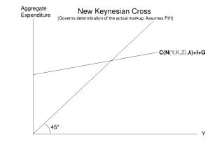
Aggregate Expenditure and Multipliers. Refer Chapter 24 (including appendix) and Chapter 25 (including appendix ) in main textbook. Topics. Consumption and income Marginal propensities to consume and save Changes in consumption and in saving Investment Net Exports Composition of spending.

E N D
Aggregate Expenditure and Multipliers Refer Chapter 24 (including appendix) and Chapter 25 (including appendix ) in main textbook
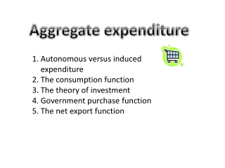
Topics • Consumption and income • Marginal propensities to consume and save • Changes in consumption and in saving • Investment • Net Exports • Composition of spending
Components of aggregate expenditure (AE) are: 1. consumption expenditure 2. Investment 3. Government purchases of goods and services 4. Net exports
Consumption Function and Saving Function 1. Consumption function • The relationship between consumption and income/disposable income, other things constant • Because consumption depends on income, it is a function of income 2. Saving function • Shows the relationship between saving and income or disposable income
Consumption Function and Saving Function • At each level of disposable income, consumption expenditure + saving always equals disposable income (Yd=C+S) • At point a, consumption expenditure is $0.75 even though the disposable income =0. This consumption expenditure is called autonomous expenditure • When C > Yd, saving is negative (dissaving) • When Yd > C, saving is positive • When Yd = C, saving = 0
Consumption expenditure • a. 450 line • 1. Each point on 45o line consumption expenditure = disposable income • 2. When consumption function lies above 45o line, C > Yd • 3. When consumption function lies above 45o line, C < Yd • 4. When consumption function intersect with 45o line, C = Yd • b. Consumption function • Along consumption function – as Yd increases, consumption expenditure also increases (positive relationship) • c. Saving function • Along saving function – as disposable income increases, saving also increases (positive relationship) 45o line (Yd=C) 5 saving 4 Consumption function 3 ● dissaving 2 1 0 3 5 4 1 2 Disposable Y Saving 1 Saving function dissaving 0 ● 1 2 3 4 5 Disposable Y -1
Marginal Propensities to Consume and Save • Marginal Propensity to Consume (MPC) 1. measures the extent to which consumption expenditure changes when disposable income changes 2. Calculated as: MPC = ∆C ∆Yd • Marginal Propensity to Save (MPS) 1. is the fraction of a change in disposable income that is saved 2. Calculated as:MPS = ∆S ∆Yd • The MPC plus MPS always equals to 1 C + S = Yd ∆C + ∆S = ∆Yd ∆C + ∆S = ∆Yd ∆Yd ∆Yd ∆Yd MPC + MPS = 1 Slopes of consumption function Slopes of saving function
Consumption expenditure 45o line (Yd=C) MPC = ∆C ∆Yd = 0.75 1 = 0.75 5 4 Consumption function ∆C = $0.75 3 ● MPS = ∆S ∆Yd = 0.25 1 = 0.25 ∆Yd = $1 2 1 0 3 5 4 1 2 Disposable Y MPC + MPS = 1 0.75 + 0.25 = 1 Saving Saving function 1 ∆S = $0.25 0 ● 1 2 3 4 5 Disposable Y -1 ∆Yd = $1
Shifts and Movements Along • There are differences between a movement along the consumption and saving function and a shift of the consumption and saving function • Movement along the consumption & saving function results from a change in income (assuming other influences on C and S are fixed) • Shift of the consumption function results from a change in one of the non-income determinants such as : Net wealth and consumption Price level Interest rate Expectations
1. Interest rate • Is a reward for savers and cost for borrowers • High interest rate - households ↑ S and ↓C. • Consumption function shifts from CF0 to CF2 while saving function shifts upward from SF0 to SF2 • Low interest rate shifts the CF upward and SF downward • 2. Net wealth • -Net wealth is the value of all assets that households own minus any liabilities, or debts owed • -A ↓ in net wealth - consumers ↓C and ↑S - CF shifts downward while SF shifts upward. • ↑ in net wealth -↑ C and ↓ S – CF shifts upward and SF shifts downward • 3. Price level • - ↑ in the price level reduces the purchasing power of wealth– households ↓ C and ↑S – CF shifts downward and SF shifts upward • - ↓ in the price level- increase the purchasing power of wealth– households ↑C and ↓S– CF shifts upward and SF shifts downward • 4. Expectations • -if expected future income ↓ - C↓ and S↑ - CF shifts downward while SF shifts upward and vice versa Consumption expenditure 45o line (Yd=C) CF1 5 CF0 4 CF2 3 2 1 0 3 5 Yd 4 1 2 Saving SF2 SF0 1 SF1 0 Yd 1 2 3 4 5 -1
Investment Function • The investment function isolates the relationship between the level of income in the economy and planned investment • Investment depends on real interest rate and the expected rate of profit (or business expectations) 1. Interest rate (negative relationship) • A decline in the rate of interest, other things remaining constant, will reduce the cost of borrowing and increase investment - investment function shifts upward • Conversely, when the interest rate increases, the planned investment function shifts downward 2. Business expectations (positive relationship) • If firms become pessimistic about profit prospects, investment will decrease at every level of income • On the other hand, if profit expectations become rosier, the investment function will shift upward
Investment Demand Curve for the Economy • Shows the inverse relationship between the quantity of investment demanded and the market interest rate, other things constant. • At lower interest rates, more investment projects become profitable for individual firms, so total investment in the economy increases.
1.1 I" 0.9 I' Planned Investment Function Real planned investment (trillions of dollars) The horizontal investment functions imply that planned investment does not vary with real disposable income, it is autonomous 1.0 I 0 2.0 4.0 6.0 8.0 10.0 12.0 14.0 Real disposable income (trillions of dollars)
Government Purchase Function • Government purchase function relates government purchases to the level of income in the economy, other things constant • Government spending or purchases do not depend directly on the level of income in the economy (autonomous or independent of income) – flat line • An ↑ in government purchases will lead to upward shift of the govt. purchase function • A ↓ in government purchases will lead to downward shift of the govt. purchase function
Net Export Function • Shows the relationship between net exports and the level of income in the economy, other things constant • Factors assumed constant along the net export function include: • The domestic price level • Price levels in other countries • Domestic and foreign Interest rates • Foreign income levels • Exchange rates between the dollar and foreign currencies
Aggregate Expenditure I + G + X + C 10 M 8 AE (C+I+G+X-M) 6 C 4 I + G + X 2 X I + G G I Real GDP 0 4 6 2 8 10
Equilibrium Expenditure and Convergence to Equilibrium • Equilibrium expenditure – is the level of aggregate expenditure that occurs when AE = RGDP (AE curve intersects with 45o line – point b • At point a – AE > RGDP →there will be a decrease in firms inventories – this will induce firms to increase production – increase in production will lead to increase in RGDP (convergence) • At point c – RGDP > AE – there will be an increase in the inventories – firms will reduce productions - RGDP↓ • Expenditure reach equilibrium through inventories adjustments Aggregate expenditure 45o 5 AE ●c b● 4 ●a 3 Equilibrium expenditure 2 1 0 3 5 6 4 1 2 RGDP
The Multiplier • When autonomous expenditure increases, AE increases and so does equilibrium expenditure and RGDP • But the increase in RGDP is larger than the change in the autonomous expenditure • Multiplier is the amount by which a change in autonomous expenditure is magnified or multiplied to determine the change in equilibrium expenditure and RGDP
The basic idea of multiplier • Suppose I ↑, so AE and RGDP also ↑ • The ↑ RGDP, increases disposable income by same amount - ↑ consumption expenditure (C ) • The initial increase in I brings an even bigger increase in AE because it induces an increase in consumption expenditure
The Multiplier 1. A $0.5 million increase in the investment lead to increases in RGDP by $2 million from 6 million to 8 million – multiplier effect 2. The multiplier is greater than 1 3. The increase in equilibrium expenditure is 4 times the increase in autonomous expenditure, Aggregate expenditure 45o 9 AEo ●e’ Multiplier = ∆ in equilibrium expenditure ∆ in autonomous expenditure = 2 0.5 = 4 d’● 8 ●e ●c’ d● 7 b’● ●c ●a’ 6 b● ●a 5 0 7 9 8 5 6 RGDP
∆Y = ∆C + ∆I (1) But change in C depends on change in MPC and RGDP ∆C = MPC X ∆Y (2) Substitute (2) into (1) ∆Y = (MPC X ∆Y) + ∆I (1-MPC) X ∆Y = ∆I ∆Y = ∆I (1-MPC) Divide both side of equation with ∆I So multiplier = ∆Y = 1 = 1 ∆I (1-MPC) MPS Suppose MPC = 0.75, so multiplier is = 1 (1-MPC) = 1/ (1-0.75) = 4
The Multiplier and Price level • To study the simultaneous determination of RGDP and the price level – need to use the AS-AD model • To understand how AD adjust we need to see the connection between the AS-AD model and the equilibrium expenditure model (AE)
Aggregate expenditure Movement along AD curve (∆P) 1. A change in the P level will shifts the AE curve, change the equilibrium expenditure and the movement along the AD curve 2. When P = 110, AE=AEo and the equilibrium expenditure=7 at point E. 3. When P ↑ to 130, AE=AE1 and the equilibrium expenditure = $6 at point a. 4. When P ↓ to 90, AE=AE2 and the equilibrium expenditure = $8 at point b. 5. Points, a, E and c on AD curve correspond to the equilibrium expenditure points a,E and c. 6. When price level are higher- AE is lower and vice versa. AE2 45o 9 AEo b ● 8 AE1 E● 7 6 a● 5 RGDP 0 7 9 8 5 6 P ↑P 130 a 110 E ↓P 90 b AD 6 7 8 RGDP
Aggregate expenditure AE1 • A Change in AD • Initially equilibrium at point a where P=110, AE=AEo and AD = Ado • An increase in autonomous expenditure (e.g a $1 million increase in investment) – shifts AE curve upward to AE1 • In the new equilibrium at point b, RGDP = $8 • Since price level did not change, ADo shift to AD1 • Main point: • When P level changes, other things remaining same, the AE shifts and there is movement along AD • When any other influence onAE curve changes, both AE and AD shift 45o 9 AEo b ● 8 7 6 a● 5 RGDP 0 7 9 8 5 6 P b 110 a 100 90 ADo AD1 6 7 8 RGDP
How do we know by how much the AD curve shifts? Depends on the multiplier. • The larger the multiplier, the larger the shift in AD curve due to changes in the autonomous expenditure • Example: A $1 million increase in the I, increases RGPD by $2 million ( from $6 to $8)
Aggregate expenditure • The Multiplier in the Short Run (↑AD) • Initially equilibrium is at point a, where AD and SRAS curves intersect, AE=AEo, P=110 and RGDP=$6 million • Suppose I ↑ by $1 million • With the price fixed at 110, AE shifts to AE1, equilibrium expenditure increases to $8million – point b. Meanwhile AD shifts rightward to AD1 by $2 million • But the price level does not remain fixed. • As the price level rises, AE shifts downward from AE1 to AE2 and new AD curve intersects the SRAS -point c – RGDP=$7.6 million and P=116 AE1 45o 9 AE2 AEo b ● 8 7.6 c 7 6 a● 5 RGDP 0 9 8 5 6 7.6 7 P SRAS c 116 110 a b 100 AD1 ADo 8 6 7 7.6 RGDP
Aggregate expenditure AE1 45o • The Multiplier in the Long Run (↑AD) • Initially equilibrium is at point a - an ↑ in the I by $1 million shifts AE to AE1 and the AD to AD1. • In the SR the economy moves to point c. • In the long run, the money wage rate rises so SRAS shift to SRAS1 and the AE curve shift back from AE2 to AEo. • In the end, the price rises (movement along AD1) and RGDP falls. • The economy moves to point E and in the long run the multiplier is zero (RGDP=PGDP). 9 AE2 AEo b ● 8 7.6 c 7 6 a● E 5 RGDP 0 9 8 5 6 7.6 7 LRAS P SRAS1 SRAS E c 116 110 a b 100 AD1 ADo 8 6 7 7.6 RGDP