Download
1 / 13
130 likes | 229 Views
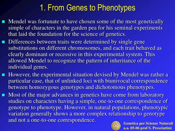
1. From Genes to Phenotypes. Mendel was fortunate to have chosen some of the most genetically simple of characters in the garden pea for his seminal experiments that laid the foundation for the science of genetics.

E N D
1. From Genes to Phenotypes • Mendel was fortunate to have chosen some of the most genetically simple of characters in the garden pea for his seminal experiments that laid the foundation for the science of genetics. • Differences between traits were determined by single gene substitutions on different chromosomes, and each trait behaved as clearly dominant or recessive in this experimental system. This allowed Mendel to recognize the pattern of inheritance of the individual genes. • However, the experimental situation devised by Mendel was rather a particular case, that of unlinked loci with biunivocal correspondence between homozygous genotypes and dichotomous phenotypes. • Most of the major advances in genetics have come from laboratory studies on characters having a simple, one-to-one correspondence of genotype to phenotype. However, in natural populations, phenotypic variation generally shows a more complex relationship to genotype and not a one-to-one correspondence.
2. Quantitative variation • The actual variation between organisms is usually quantitative, not qualitative. Wheat plants in a cultivated field or wild asters at the side of the road are not neatly sorted into categories of “tall” and “short”, any more than humans are neatly sorted into categories of “black” and “white”. Height, weight, shape, color, metabolic activity, reproductive rate, and behavior are characteristics that vary more or less continuously over a range. • Even when the character is intrinsically countable (such as eye facet or bristle number in Drosophila), the number of distinguishable classes may be so large that the variation is nearly continuous.
3. Mendelian traits are the exception rather than the rule • If we consider extreme individuals - say, a corn plant 8 feet tall and another one 3 feet tall - a cross between them will not produce a Mendelian result. • Such a corn cross will produce plants about 6 feet tall, with some clear variation among siblings. • The F2 from selfing the F1 will not fall into two or three discrete height classes in ratios of 3:1 or 1:2:1. • Instead, the F2 will be continuously distributed in height from one parental extreme to the other. • This behavior of crosses is not an exception; it is the rule for most characters in most species.
4. Crosses between pure lines The inheritance of corolla length in Nicotiana longiflora. Results are shown as the percentage frequencies with which individuals fall into classes, each covering a range of 3 millimeters in corolla length. This grouping is quite artificial and the apparent discontinuities are spurious: corolla length actually varies continuously. The means of F1 and F2 are intermediate between those of the parents. The means of the four F2 families are correlated with the corolla length of the F2 plants from which they came, as indicated by the arrows. Variation in parents and Fl is all nonheritable, and hence is less than that in F2, which shows additional variation arising from the segregation of the genes concerned in the cross. Variation in F3 is, on the average, less than that of F2 but greater than that of parents and F1. Its magnitude varies among the different F2's according to the number of genes that are segregating.
5. Continuity of phenotypic traits under Mendelian inheritance • Mendel obtained his simple results because he worked with horticultural varieties of the garden pea that differed from one another by single allelic differences that had drastic phenotypic effects. Had Mendel conducted his experiments on the natural variation of the weeds in his garden, instead of abnormal pea varieties, he would never have discovered Mendel’s laws. In general, size, shape, color, physiological activity, and behavior do not assort in a simple way in crosses. • The fact that most phenotypic characters vary continuously does not mean that their variation is the result of some genetic mechanisms different from the Mendelian genes with which we have been dealing. • The continuity of phenotype is a result of two phenomena. • First, each genotype may show such a a wide range of phenotypic values that, as a result, the phenotypic differences between genotypic classes become blurred, and we are not able to assign a particular phenotype unambiguously to a particular genotype. • Second, many segregating loci may have alleles that make a difference to the phenotype being observed.
6. An apparently insoluble controversy • Soon after the rediscovery of Mendel’s work, it was debated whether continuously varying traits were inherited in fundamentally different ways from discrete traits. Many argued for a form of blending inheritance that did not involve particulate inheritance (discrete genes). • The claims of the Mendelians, championed by Bateson, were resisted by biometricians. Biometricians allowed that Mendelian genes might explain a few rare abnormalities or curious quirks, but pointed out that most of the characters likely to be important in evolution (body size, build, strength, skill in catching prey or finding food) were continuous or quantitative characters and not amenable to Mendelian analysis. You cannot define their inheritance by drawing pedigrees and marking in the affected people, because we all have these characters, only to different degrees. Mendelian analysis requires dichotomous characters (characters like extra fingers, that you either have or don't have). • The controversy ran on, heatedly at times, until 1918. That year saw a seminal paper by RA Fisher demonstrating that continuous characters governed by a large number of independent Mendelian factors (polygenic characters) would display precisely the quantitative variation and family correlations described by the biometricians.
7. Two traditions in human genetics • In principle Fisher's description of polygenic inheritance unified genetics. This was indeed generally true for the genetics of experimental organisms or farm animals. In human genetics, however, studies of Mendelian and quantitative characters tended to continue as separate traditions, and until very recently few investigators felt at home in both worlds. • The spectacular advances of 1970-1990 were entirely in Mendelian genetics, whilst investigation of nonmendelian characters remained largely limited to statistical studies of family resemblances. Geneticists from the Mendelian tradition were often reluctant to get involved in these studies, partly because of the complex statistical methodology and no doubt also because of a feeling that they were a poor investment of research effort compared to mapping and cloning genes for mendelian characters. • Recent developments have finally brought together the study of Mendelian and complex human phenotypes. Automation is allowing genetic analysis and sequencing on a scale scarcely imagined ten years ago. This has had two consequences. Most human genes are now identified, so that molecular geneticists are looking for fresh fields to conquer. At the same time, marker studies can now be done on a scale that is probably large enough to deliver the statistical power needed to detect individual quantitative trait loci and susceptibility loci. • Given the overwhelming preponderance of non-Mendelian conditions in human disease, molecular dissection of complex phenotypes is widely seen as the next frontier in human genetics.
8. A basic quantitative model Suppose that five equally important loci affect the number of flowers that will develop in an annual plant and that each locus has two alleles (call them + and -). For simplicity, also suppose that there is no dominance and that a + allele adds one flower, whereas a - allele adds nothing. Thus, there are 35 = 243 different possible genotypes [three possible genotypes (+ / +, + -, and - / -) at each of five loci], ranging from but there are only 11 phenotypic classes (10, 9, 8, . . . , 0) because many of the genotypes will have the same numbers of + and − alleles. For example, although there is only one genotype with 10 + alleles and therefore an average phenotypic value of 10, there are 51 different genotypes with 5 + alleles and 5 − alleles; for example, Thus, many different genotypes may have the same average phenotype. At the same time, because of environmental variation, two individuals of the same genotype may not have the same phenotype. This lack of a one-to-one correspondence between genotype and phenotype obscures the underlying Mendelian mechanism.
9. Human skin color as an example of polygenic inheritance In human, no equivalent may exist of a pure genetic line; however, in the case of skin color, some populations have been naturally selected for an extreme phenotype, black or white. This does not guarantee that these “lines” are pure, but it is certainly true that the differences between the extreme populations are much higher than differences within populations. Subjects born from parents of the two opposite populations show an intermediate skin color; the distribution of skin color in the F2 individuals suggests that three or four loci are involved. Skin color is measured by reflectance of light at wavelength 685 nm. F2 distributions are those expected according to different hypotheses about the number of genes involved
10. Between Mendelian and quantitative genetics Using the concepts of distribution, mean, and variance, we can understand the difference between quantitative and Mendelian genetic traits. Suppose that a population of plants contains three genotypes, each of which has some differential effect on growth rate. Furthermore, assume that there is some environmental variation from plant to plant. For each genotype, there will be a separate distribution of phenotypes with a mean and a standard deviation that depend on the genotype and the set of environments. Suppose that these distributions look like the following height distributions:
11. Mixed distributions Finally, assume that the population consists of a mixture of the three genotypes but in the unequal proportions 1:2:3 (a/a: A/a: A/A). Then the phenotypic distribution of individuals in the population as a whole will look like the black line in the following figure: This is the result of summing the three underlying separate genotypic distributions, weighted by their frequencies in the population. The mean of the total distribution is the average of the three genotypic means, again weighted by the frequencies of the genotypes in the population. The variance of the total distribution is produced partly by the environmental variation within each genotype and partly by the slightly different means of the three genotypes.
12. Distribution of acid phosphatase activity The human red cell acid posphatase (ACP1) genetic polymorphism offers a good example of the complementary points of view of Mendelian and quantitative genetics. When H. Harris and D. Hopkinson sampled an English population in the search of genetic polymorphisms, they found that three allelic forms were present for ACP1, A, B, and C, at different frequencies. The three alleles combine to form six genotypes, and these show significant variation in enzyme activity; however none of the genotypes can be unambiguously identified based on the measured activity
13. Variance of ACP1 activity explained by genetic differences among individuals This Table shows the mean activity, the variance in activity, and the population frequency of the six genotypes. About half of the variance in activity in the total distribution (607.8) is explained by the average variance within genotypes (310.7), so half (607.8 - 310.7 = 297.1) is accounted for by the variance between the means of the six genotypes. Although much of the variation in activity is explained by the mean differences between the genotypes, there remains variation within each genotype that may be the result of environmental influences or of the segregation of other, as yet unidentified, genes.