Download
1 / 36
370 likes | 530 Views
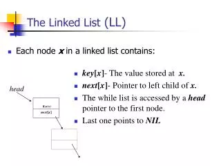
The Linked List (LL). Each node x in a linked list contains:. key [ x ] - The value stored at x. next [ x ] - Pointer to left child of x. The while list is accessed by a head pointer to the first node. Last one points to NIL. head. Key(x). next [ x ].

E N D
The Linked List (LL) • Each node x in a linked list contains: • key[x]- The value stored at x. • next[x]- Pointer to left child of x. • The while list is accessed by a head pointer to the first node. • Last one points to NIL head Key(x) next[x]
Inserting the element into LL • Find a place for it. • Point “new’s” next to the next. • Point “previous’s”next to new. head head head Key(x) New element Key(x) Key(x) next[x] next[x] next[x] Key(x) Key(x) Key(x) next[x] next[x] next[x]
Key(x) next[x] Key(x) next[x] Removing the element from LL • Find the element. • Point “previous’s” next to the next. • Point previous to new. head head head Deleted element Key(x) Key(x) next[x] next[x] Key(x) Key(x) next[x] next[x]
Reporting in sorted order • If you keep the list sorted at all the times the reporting it in sorted order is as simple as iterating through the list and reporting the elements as you encounter them.
Heap • A heap is a binary tree storing keys, with the following properties: • partial order: • key (child) < key(parent) • left-filled levels: • the last level is left-filled • the other levels are full X T O G S M N A E R B I
Heap Representations 1 X 3 2 • left_child(i)= 2i • right_child(i) = 2i+1 • parent(j) = j div 2 T O 4 5 6 7 G S M N 9 10 8 11 12 A E R B I
Heap Insertion X T O X G S M N T O A E P R B I G S M N X A E P R B I T O • Add the key in the next available spot in the heap. • Upheap checks if the new node is greater than its parent. If so, it switches the two. • Upheap continues up the tree G S P N A E M R B I
Heap Insertion X X T O T P G S P N G S O N A E M R B I A E M R B I
Heap Insertion X • Upheap terminates when new key is less than the key of its parent or the top of the heap is reached. • (total #switches) <= (height of tree- 1) =log n T P G S O N A E M R B I
Heapify Algorithm • Assumes L and R sub-trees of i are already Heaps and makes It's sub-tree a Heap: Heapify(A,i,n) If (2i<=n) & (A[2i]>A[i]) Then largest=2i Else largest=i If (2i+1<=n) & (A[2i+1]>A[largest]) Then largest=2i+1 If (largest != i) Then Exchange (A[i],A[largest]) Heapify(A,largest,n) Endif End Heapify
Extracting the Maximum from a Heap: X 1 • Here is the algorithm: Heap-Extract-Max(A) Remove A[1] A[1]=A[n] n=n-1 Heapify(a,1,n) End Heap-Extract-Max T P 2 G S O N A E M R B I M 3 T P G S O N A E R B I
Building a Heap • Builds a heap from an unsorted array: Build_Heap(A,n) For i=floor(n/2) down to 1 do Heapify(A,i,n) End Build_Heap • Example: 4 A 1 3 i 2 16 9 10 14 8 7
Building a Heap (cont’d.) 4 4 i 1 3 1 3 i 2 16 9 10 16 9 10 14 14 8 i 8 7 2 7 4 4 i 16 10 1 10 14 9 3 16 9 3 7 14 2 8 1 2 8 7
Building a Heap (cont’d.) 16 14 10 8 9 3 7 2 4 1
Finding an Element • Must look at each element of the array: For i=1 to n do if A(i) == b break; • Example: 1 X 3 2 T O 4 5 6 7 G S M N 9 10 8 11 12 A E R B I A
Removing an Element • Must find it first • After that similar to remove Max Remove A[i] A[i]=A[n] n=n-1 Heapify(a,i,n) 1 X 3 2 T O 4 5 6 7 G S M N 9 10 8 11 12 A E R B I A
Removing an Element 1 1 X X 3 3 2 2 T O T O 4 5 4 5 6 7 6 7 G I M N G S M N 9 10 9 10 8 11 8 11 12 A E A E R B R B I 1 X 3 2 T O 4 5 6 7 G R M N 9 10 8 11 A E I B
The Binary Search Tree (BST) • Each node x in a binary search tree (BST) contains: • key[x]- The value stored at x. • left[x]- Pointer to left child of x. • right[x]- Pointer to right child of x. • p[x]- Pointer to parent of x. x P(x) Key(x) left[x] right[x]
BST- Property • Keys in BST satisfy the following properties: • Let x be a node in a BST: • If y is in the left subtree of x then: key[y]<=key[x] • If y is in the right subtree of x then: key[y]>key[x]
Example: • Two valid BST’s for the keys: 2,3,5,5,7,8. 2 5 3 3 7 7 5 8 2 5 8 5
In-Order Tree walk • Can print keys in BST with in-order tree walk. • Key of each node printed between keys in left and those in right subtrees. • Prints elements in monotonically increasing order. • Running time?
In-Order Traversal Inorder-Tree-Walk(x) 1: If x!=NIL then 2:Inorder-Tree-Walk(left[x]) 3:Print(key[x]) 4:Inorder-Tree-Walk(right[x]) What is the recurrence for T(n)? What is the running time?
In-Order Traversal • In-Order traversal can be thought of as a projection of BST nodes on an interval. • At most 2d nodes at level d=0,1,2,… 5 3 7 5 2 8 2 3 5 5 7 8
Other Tree Walks Preorder-Tree-Walk(x) 1: If x!=NIL then 2:Print(key[x]) 3: Preorder-Tree-Walk(left[x]) 4:Preorder-Tree-Walk(right[x]) Postorder-Tree-Walk(x) 1: If x!=NIL then 2:Postorder-Tree-Walk(left[x]) 3:Postorder-Tree-Walk(right[x]) 4:Print(key[x])
Searching in BST: • To find element with key k in tree T: • Compare k with the root • If k<key [root[T ]] search for k in the left sub-tree • Otherwise, search for k inthe right sub-tree Search(T,k) 1: x=root[T] 2:If x=NIL then return(“not found”) 3: If k=key[x] then return(“found the key”) 4: If k< key[x] then Search(left[x],k) 5: else Search(right[x],k)
Examples: • Search(T,11) • Search(T,6) 5 5 3 10 3 10 7 2 5 11 7 2 5 11 4 4
BST Insertion • Basic idea: similar to search. • BST-Insert: • Take an element z (whose right and left children are NIL) and insert it into T. • Find a place where z belongs, using code similar to that of Search. • Add z there.
Insert Key BST-Insert(T,z) 1: y=NIL 2: x=root[T] 3: While x!=NIL do 4: y=x; 5: if key[z]<key[x] then 6: x=left[x] 7: else x=right[x] 8: p[z]=y 9: if y=NIL the root[T]=z 10: else if key[z]<key[y] then left[y]=z 11: else right[y]=z Insert(T,8) 5 3 10 7 2 5 11 8 4
Locating the Minimum 5 BST-Minimum(T) 1: x=root[T] 2:While left[x]!=NIL do 3: x=left[x] 4: return x 3 10 7 2 5 11 8 4
Application: Sorting • Can use BST-Insert and Inorder-Tree-Walk to sort list of nnumbers BST-Sort 1: root[T]=NIL 2:for i=1to n do 3:BST-Insert(T,A[i]) 4: Inorder-Tree-Walk(T) Sort Input: 5, 10, 3, 5, 7, 5, 4, 8 5 3 10 5 5 5 7 10 4 8 Inorder Walk: 3, 4, 5, 5, 7, 8, 10
Successor Given x, find node with smallest key greater than key[x]. Here are two cases depending on right subtree of x. • Successor Case 1: • The right subtree of x is not empty. Successor is leftmost node in right subtree. That is, we must return BST-Minimum(right[x]) x 5 3 10 5 7 Successor 4 8
Successor • Successor Case 2: The right subtree of x is empty. Successor is lowest ancestor of x. Observe that, “Successor” is defined as the element encountered by inorder traversal. Successor BST-Successor(x) 1: If right[x]!=NIL then 2:return BST-Minimum(right[x]) 3: y=p[x] 4:While (y!=NIL) and (x=right[y]) 5: x=y 6: y=p[y] 7: return y Running time? 5 1 10 3 7 x 8
Deletion • Delete a node x from tree T: • Case 1: x has no children. A A B D B D C x
Deletion: • Case 2: x has one child (call it y). Make p[x] to replace y instead of x as its child, and make p[x] to be p[y]. A A B D C D x C
Deletion: • Case 3: x has two children: • Find its successor ( or predecessor) y. • Remove y. (Note y has at most one child, why?) • Replace x by y. A C x B D B D C y
Delete Procedure BSFT-Delete(T, z) 1: If (left[z]=NIL) or (right[z]=NIL) then 2: y=z 3: else y=BST-Successor(z) 4:Ifleft[y]!=NIL then 5: x=left[y] 6: else x=right[y] 7: If x!=NIL then p[x]=p[y] 8: If p[y]=NIL then root[T]=x 9: else if y=left[p[y]] then left[p[y]]=x 10:else right[p[y]]=x 11: if y!=z then key[z]=key[y] 12: return y