Forest Mitigation Strategy: REDD

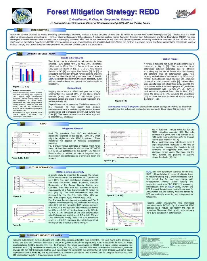
1. INTRODUCTION Ecosystem services provided by forests are widely acknowledged. However, the loss of forests amounts to more than13 million ha per year with various consequences [1]. Deforestation is a major driver of climate change accounting for ~ 12% of global anthropogenic CO2 emissions. A mitigation strategy named Reduction Emission from Deforestation and forest Degradation (REDD) has been developed to tackle emissions due to forest loss in developing countries. REDD will be the main core in any post-2012 climate agreement according to the final document of the 15th and 16th UN Conference of the Parties. Nonetheless, REDD's implementation presents several political and scientific challenges. Within this context, a review of current and future deforestation estimates in terms of surface change, and carbon fluxes has been prepared. An overview of these data is presented here. CURRENT DEFORESTATION REDD FUTURE SCENARIOS SUMMARY AND FUTURE WORK Historical deforestation surface changes and relative CO2 emission estimates were presented. The work found in the literature is limited and data are uncertain. Estimates of REDD mitigation potential vary significantly. Climate feedbacks in particular might counterbalance REDD's benefits [15, 16]. Furthermore, the future contribution of REDD in 5 major emitter countries was estimated as in [17]. Deforestation slow-down at 1%, 3%, 5%, 10%, 20% and 50% were considered to introduce CO2 emission savings into the RCP 8 scenario. Further work is necessary to investigate the uncertainties of these findings. A dynamic global vegetation model (ORCHIDEE) was recently used to estimate the permissible land use emissions for assigned future atmospheric CO2 stabilization targets [19] and compared to IAM fluxes. Forest Mitigation Strategy: REDD C. Arcidiacono, P. Ciais, N. Viovy and N. Vuichard Le Laboratoire des Sciences du Climat et l'Environnement (LSCE), Gif-sur-Yvette, France Trends in Forest Area Carbon Fluxes Total forest loss is attributed to deforestation in Latin America, ~60% (Brazil 48%), in Asia, 30% (Indonesia 13%), and in Africa 5% [1]. Trends in forest area in 1990-2010 are shown in Fig. 1 [1, 2, 3]. New revised data from FAO [1] are higher than before [2]. In [3], a consistent methodology through remote sensing provides for the first time the global gross cover loss of forests. REDD will greatly benefit from this latest approach, but it will also need to know the dynamics of carbon cycle in forests [4]. A review of historical net fluxes of carbon from LUC is presented in Fig. 2 [8]. This shows the broad differences between estimates due to different accounting e.g the fate of forests after the clearing, and different rates of deforestation used. More recently, revised rates of deforestation by FAO through revised methodologies have lowered CO2 estimates compared to the previous study [9]. Nevertheless, large uncertainties still affect these data. In 2008, the contribution to the total anthropogenic CO2 emissionsfrom deforestation was ~1.2 GtC yr-1, i.e. ~12% of total emissions (updated from 17% in IPCC 2007) within the range of 6–17% including the uncertainty [10]. In 2009, the flux estimate fell further reaching 1.1 GtC yr-1 [11]. Figure 1. [1, 2, 3] Carbon Stock Method uncertainties Ground based survey: labour intensive and time consuming, thus expensive. Data present large uncertainties. Nowadays, remote sensing metric are also integrated to refine forest classification. FAO data, being based on country statistics, inform on local level trends, and on net deforestation. However, REDD programs require gross deforestation data. Remote sensing: highly accurate, same criteria applied worldwide, and possibility for improvement. Mapping carbon stock is difficult and gives rise to large uncertainties [5]. Around 80% of the above ground biomass (AGB), and 40% of the below ground terrestrial carbon are found in the forest vegetation and soil respectively [6]. Tropical forests store more than 320 billion tonnes of C [5]. However, no high quality field biomass measurements exist at sufficient spatial extent. Remote sensing could aid to measure directly AGB where most C lies [7]. This would represent an alternative approach to estimate CO2 emissions. Figure 2. [8] Consequence for REDD programs: the maximum carbon savings are likely to be lower than expected, but the inclusion of peatlands might add up to 3% of global CO2 emissions [10]. r Mitigation Potential Fig. 4 illustrates various estimates for the REDD mitigation potential [13]. The only estimate at a global level is by Sathaye et al. [14], while most projections refer to tropical nations (see legend in Fig. 4). These projections vary notably and present large uncertainties especially at the end of the century. However, the literature is not conflicting in suggesting that REDD will introduce carbon gains. The main risk for REDD success lies probably in positive climate feedbacks [15, 16]. Most CO2 emissions from LUC are attributed to developing countries in the tropics, ~96% [9], which might be eligible to claim REDD incentives. These incentives will depend on historical deforestation baselines. Fig. 3 shows various estimates of tropical moist forest area (106 ha) time series for 63 countries 1973–2010 [12, 1, 3]. As questioned by the author [12], none of these studies is reliable to infer a long-term trend (baseline) in tropical forest area if errors are taken into account. Figure 3. [1, 3, 12] Figure 4. [13] RCPs, four new benchmark scenarios for the next IPCC [18] are labelled in terms of ultimate levels of radiative forcing. Fig. 7 shows contrasted RCP 8 IAM model flux for land use change with corresponding results (same forcing and vegetation map) from ORCHIDEE [19] accounting deforestation only. In REDD terms, RCP2.6 and RCP 8 project the decline of tropical forest area (~ 20%) within the XXI century, while the remaining RCP are optimistic expecting an enlargement of forest area. REDD: a simple case study A simple study is presented to analyze the future REDD contribution to the abatement of CO2emissions as in [17]. Five main contributors countries to LUC flux were considered: Brazil, Indonesia, Republic Democratic of the Congo, Nigeria, Bolivia, and Colombia. Their total area was assumed to decline monotonically at a fixed historical rate (6 million ha yr-1) (Fig. 5). The total deforestation rate was decreased by 1%, 3%, 5%, 10%, 20%, 50% per year after the post Kyoto Protocol year, 2012. Fig. 5 shows the net changes scenarios, and Fig. 6 displays the corresponding CO2 emissions for various rates. By 2100, the cumulative LUC emission amounts to ~5 GtC in a BAU scenario. This contribution lowers by 40% to ~3 GtC at 1% slowdown, and by 60% to ~2 GtC at 3% slowdown of the total deforestation rate. Emissions are abated to ~1 GtC at both 5% and 10% slowdowns. Finally, 20%, and 50% slowdowns result in ~0.5 GtC emissions. Overall findings fallat the higher end of Poulter's results in Fig. 4. Figure 7. [18, 19]. Figure 5. Possible REDD interventions were introduced tentatively under RCP 8.5. Fig. 8. shows that REDD options could reduce significantly the rate of emissions. These are offset by mid century already for a 10% slowdown in deforestation. Figure 6. Figure 8. [18] References [1] FAO 2010, Forest Resource Assesment [2] FAO 2006, State of the World Forest [3] Hansen et al. 2010, PNAS 107 19 8650 [4] Kurz 2010 PNAS 107 20 9025 [5] Gibbs et al. 2007, Environ. Res. Lett. 2 045021 [6] Houghton J. 2009, Global Warming 49 [7] Baccini et al. 2008, Environ. Res. Lett. 3 045011 [8] Ramankutty et al. 2007, Glob. Ch. Biology, 51 [9] Houghton R.A. 2010,Tellus (2010), 62B, 337; Tellus 55B 378; 2008http://cdiac.ornl.gov/trends/landuse/ houghton/houghton.html [10]Van der Werf 2009, Nat. Geosci. 2 [11] Friedlingstein et al. 2010, Nature Geoscience 3 811–812. [12] Grainger 2008, PNAS 105 2 and references therein [13] Arcidiacono-B et al. 2010, Proc. Env. Sci. in publication and references therein [14] Sathaye et al. 2007, En. J. 3 127 [15] Gumpenberger et al. 2010, Environ. Res. Lett. 5 014013 [16] Poulter et al. 2010, Glob. Change Biol. 16 2062 [17] Mollicone et al. 2007, Environ. Res. Lett. 045024 [18] http://www.iiasa.ac.at/web-apps/tnt/RcpDb and references therein [19] Noblet et al. 2011, unpublished.