Download
1 / 15
150 likes | 227 Views
GW Backgound from extragalactic Double Neutron Stars. Tania Regimbau Virgo/ARTEMIS-OCA. Plan. Monte Carlo simulations in the frequency band of: Ground-based interferometers: last 1000 s before the LSO LISA band: low frequency inspiral signal.

E N D
GW Backgound from extragalactic Double Neutron Stars Tania Regimbau Virgo/ARTEMIS-OCA
Plan Monte Carlo simulations in the frequency band of: • Ground-based interferometers: last 1000 s before the LSO • LISA band: low frequency inspiral signal
The GW Stochastic Background 10-43s: gravitons decoupled (T = 1019 GeV) • Two contributions: • cosmological:signature of the early Universe inflation, cosmic strings, phase transitions… • astrophysical:superposition of all the sources since the beginning of the stellar activity: Compact binairies, supernovae, BH ring down, supermassive BH … • characterized by the energy density parameter: 300000 yrs:photonsdecoupled (T = 0.2 eV)
Astrophysical Stochastic Backgrounds • To model astrophysical backgrounds one needs to know: • The cosmological model (H0, Wm , Wn): • 737 cosmology: flat Einstein de Sitter Universe with h0=0.7, Wm=0.3, Wn=0.7 • The source rate dR(z) • The individual energy spectral density
Random selection of zf zb = zf - Dz If zb < 0 x N=106 (uncertainty on Wgw <0.1%) Random selection of t Compute zc If zc < z* Compute fn0 Last thousands seconds before the last stable orbit: 96% of the energy released, in the range [10-1500 Hz] Ground-based interferometer frequency band • redshift of formation of massive binaries (Coward et al. 2002) • redshift of formation of NS/NS • coalescence time • redshift of coalescence • observed fluence
Detection Regimes The duty cycle characterizes the nature of the background. <t> = 1000 s, which corresponds to 96% of the energy released, between 10-1500 Hz • D >1: continuous (z>0.1, 96%) The time interval between successive events is shortcompared to the duration of a single event • D <1: shot noise(z<0.01) The time interval between successive events is long compared to the duration of a single event • D ~1: popcorn (0.01<z<0.1) The time interval between successive events is of the same order as the duration of a single event
Detection • Because the stochastic background cannot be distinguished from the instrumental noise background, the optimal detection strategy is to correlate the outputs of two (or more) detectors. hypothesis: • isotropic, gaussian, stationnary • signal and noise, detector noises uncorrelated Cross correlation statistic: • combine the signal outputs using an optimal filter to optimize the signal to noise ratio Signal to noise ratio: 2 colocated/coaligned advanced detectors (LIGO ad): S/N ~0.65 • 2 colocated/coaligned 3rd generation detectors (EGO):S/N ~10
Random selection of zf zb = zf - Dz If zb < 0 Random selection of t x N=106 Compute ze Compute fn0 LISA frequency band • redshift of emission • observed fluence
Summary • GBased interferometers (1000s before LSO): • 3 regimes: resolved (z<0.01), popcorn (0.01<z<0.1), continuous (z>0.1) • continuous contribution reaches a maximum of around 930 Hz • S/R~0.65 (~10) for second (third) generation of interferometers • LISA band (low frequency inspiral phase): • may dominate the LISA instrumental noise between 0.7-6 mHz (or 0.3-10 mHz for the less conservative estimate), and the galactic double white dwarf confusion noise after 2 mHz. • however, the resulting reduction in the sensitivity should be less than a factor 4 and thus shouldn't affect significantly signal detection.
Random selection of zf zb = zf - Dz If zb < 0 Random selection of t x N=106 Compute ze Compute fn0 LISA frequency band • observed frequency range • redshift of emission • observed fluence • number of sources present today