Download
1 / 23
230 likes | 362 Views
Effects of Grid Resolution and Perturbations in Meteorology and Emissions on Air Quality Simulations Over the Greater New York City Region.

E N D
Effects of Grid Resolution and Perturbations in Meteorology and Emissions on Air Quality Simulations Over the Greater New York City Region Christian Hogrefe1,2,*, Prakash Doraiswamy2, Brian Colle3, Ken Demerjian2, Winston Hao1, Mark Beauharnois2, Michael Erickson3, Matthew Souders3, and Jia-Yeong Ku1 1New York State Department of Environmental Conservation, 625 Broadway, Albany, NY 2Atmospheric Sciences Research Center, University at Albany, 251 Fuller Road, Albany, NY 3School of Marine and Atmospheric Sciences, Stony Brook University, Stony Brook, NY *Now at U.S. Environmental Protection Agency, RTP, NC Acknowledgments and Disclaimer: The model simulations analyzed in this presentation were performed by the New York State Department of Environmental Conservation (NYSDEC) with partial support from the New York State Energy Research and Development Authority (NYSERDA) under agreement #10599. The views expressed here do not necessarily reflect the views or policies of U.S. EPA, NYSDEC or NYSERDA. U.S. Environmental Protection Agency
Objectives • Quantify and compare the relative impacts of perturbations in meteorology, emissions, and grid resolution on CMAQ predictions of 8-hr daily maximum O3 and 24-hr average PM2.5 • How do these impacts vary in time and space? • How do these factors vary on a diurnal scale for wintertime PM2.5? • Evaluate the overall ensemble and three sub-ensembles (meteorology, emissions, and grid resolution) using probabilistic metrics • How well do these ensembles capture threshold exceedance probabilities? U.S. Environmental Protection Agency
Overview • Meteorological Perturbations (12 members): • Use of twelve MM5 and WRF weather forecasts from the Stony Brook ensemble system to drive CMAQ4.7.1 • 36 km / 12 km domains • Emission Perturbations (100 members): • Use of a single MM5 ensemble member to drive CMAQ4.7.1 configured with DDM to calculate sensitivities towards perturbations in NOx, VOC, and PM2.5 emissions • The NOx, VOC, and PM2.5 emission perturbations considered in this study were sampled from a uniform distribution representing an uncertainty range of +/-50% • 36 km / 12 km domains • Grid Resolution Perturbations (81 members): • Use of WRF-UCM 36km/12km/4km/1.33km to drive CMAQ4.7.1 • Consider the 81 1.33 km cells within each 12 km cell as perturbations from the 12km base case • Caveat: There is no common “base” setup between these three sets of simulations U.S. Environmental Protection Agency
Overview (Continued) All simulations were performed for August 1 – 31, 2010 and January 1- February 15, 2011 All analysis was performed for the smallest domain common to all simulations, i.e. the 1.33 km modeling domain (details next slide) Analysis focuses on daily maximum 8-hr O3 and 24-hr average PM2.5 U.S. Environmental Protection Agency
Location of Hourly O3 and PM2.5 Monitors Within the Analysis Domain (Identical to the 1.33 km Domain Shown on the Left) 36 km , 12 km, 4 km, and 1.33 km Domains Used for the Grid Resolution Ensemble Simulations Note: the meteorological and emission perturbation ensemble simulations were performed on nested 36 km / 12km domains. While similar in spatial extent to the 36 km / 12 km domains shown above, a slightly different projection center was used and the 12 km outputs from these simulations were regridded to the analysis domain shown on the right U.S. Environmental Protection Agency
Example: Observed and Ensemble Daily Maximum 8-hr O3, August 2010 Stratford, CT Manhattan, NY • Qualitatively, ozone fluctuations during August 2010 were captured by the various ensembles • Grid resolution effects are more pronounced for the Manhattan monitor than the CT monitor • More generally, the effects of the various ensemble perturbations vary over space and time U.S. Environmental Protection Agency
Ensemble Coefficient of Variation (CV), 8-Hr DM O3, August 2010 (For each grid cell and day, calculated CV as ensemble standard deviation / ensemble mean, then calculated monthly average CV for each grid cell) Meteorological Ensemble Emissions Ensemble Grid Resolution Ensemble • All ensembles have the largest CV over NYC (this is also true when looking at the ensemble standard deviation or ensemble range) • Average CV all O3 Monitors: Meteorology 11.0%, Emissions 6.5%, Grid Resolution 4.3% U.S. Environmental Protection Agency
Relative Rank of Various Perturbations Measured by the Coefficient of Variation, Averaged over August 2010, 8-hr DM O3 Meteorology NOx/VOC Emissions Grid Resolution • Meteorological perturbations are the dominant factor for the entire analysis domain • The ranking shown here is specific to the pollutant, time period, domain, and ensemble configuration used in this study U.S. Environmental Protection Agency
Example: Observed and Ensemble 24-Hr Average PM2.5, Jan/Feb 2011 Holtsville, NY Manhattan, NY • While mean observed PM2.5 levels appear to be roughly captured by all ensembles for the Holtsville monitor, they are overestimated for the Manhattan monitor • Grid resolution effects are more pronounced for the Manhattan monitor than the Holtsville monitor U.S. Environmental Protection Agency
Ensemble Coefficient of Variation (CV), 24-Hr Average PM2.5, Jan/Feb 2011 (For each grid cell and day, calculated CV as ensemble standard deviation / ensemble mean, then calculated monthly average CV for each grid cell) Meteorological Ensemble Emissions Ensemble Grid Resolution Ensemble • The primary PM2.5 emission and grid resolution ensembles have the largest CV over NYC • Average CV all PM2.5 Monitors: Meteorology 17.8%, Emissions 15.9%, Grid Resolution 14.4% • The variations introduced by grid resolution effects show larger spatial gradients than those introduced by emission and meteorological perturbations U.S. Environmental Protection Agency
Relative Rank of Various Perturbations Measured by the Coefficient of Variation, Averaged over Jan/Feb 2011, 24-Hr Average PM2.5 Meteorology Primary PM2.5 Emissions Grid Resolution • In the 12km grid cells located over NYC, primary PM2.5 emission perturbations and grid resolution have a bigger impact than meteorological perturbations for simulated PM2.5 during this wintertime period. • The ranking shown here is specific to the pollutant, time period, domain, and ensemble configuration used in this study U.S. Environmental Protection Agency
Ratio of Purely Primary PM2.5 (EC, POA, A25) to Total PM2.5 (lower bound of total primary PM2.5 - primary sulfate and nitrate were not tracked separately in these model runs) Time Series of Primary/Total PM2.5 (Distribution Across All Sites) Average Primary/Total PM2.5, Jan/Feb 2011 • Primary PM2.5 species account for roughly 50% of total PM2.5 • perturbations in primary PM2.5 emissions and grid resolution (affecting the spatial distribution of these emissions) can have a strong impact on total PM2.5 predictions over the NYC area for this time period • examine role of emissions, meteorology, and grid resolution from a diurnal perspective U.S. Environmental Protection Agency
Diurnal Cycles of PM2.5 Emissions, PBL Height, and Ventilation Coefficient (VC) Average Jan 1 – Feb 15, 2011, All PM2.5 Sites, 12km “Emission Ensemble” Base Simulation • There is a lag between the diurnal cycles of PM2.5 emissions on the one hand and PBL height and VC on the other hand • CMAQ PM2.5 concentrations are expected to be particularly sensitive towards PM2.5 emission perturbations during early morning and late afternoon PM2.5 Emissions PBL Height Ventilation Coefficient U.S. Environmental Protection Agency
Subgrid Variability of PM2.5 Emissions, PBL Height, and Ventilation Coefficient (VC) Average Diurnal Cycle Jan 1 – Feb 15, 2011, Variability of 81 1.33 km Grid Cells Within Each 12 km Grid Cell Corresponding to a PM2.5 Monitoring Site Median and Interquartile Range Only Full Ensemble Range • Moving from 12 km to 1.33 km grid spacing introduces more subgrid variability for PM2.5 emissions than PBL height or VC for this domain and wintertime study period • The subgrid distribution of PM2.5 emissions is assymetric • This subgrid scale variability of PM2.5 emissions likely has a significant impact on the spread of the PM2.5 concentrations predicted by the grid resolution ensemble, especially during early morning and late afternoon U.S. Environmental Protection Agency
Diurnal Variation of Ensemble Spread for PM2.5 Concentrations Average Diurnal Cycle Jan 1 – Feb 15, 2011, all PM2.5 Monitoring Site Full Ensemble Range Median and Interquartile Range Only • The range of the PM2.5 concentrations predicted by the two ensembles directly or indirectly affecting emissions (i.e. the PM2.5 emissions ensemble and grid resolution ensemble) exceeds the range predicted by the meteorological ensemble, especially during early morning and late afternoon • As shown previously, all ensembles are biased high with respect to observations U.S. Environmental Protection Agency
Probabilistic Model Evaluation U.S. Environmental Protection Agency
Talagrand Diagrams for Probabilistic Forecasts of 8-hr DM O3, August 2010 • All ensembles are underdispersed and exhibit some bias towards overprediction U.S. Environmental Protection Agency
Reliability Diagrams for Probabilistic Forecasts of 8-hr DM O3 > 60 ppb August 2010 • All ensembles show better probabilistic skill than climatology for this exceedance threshold which corresponds to the AQI transition from green to yellow • Brier Skill Scores for a range of exceedance thresholds are shown on the next slide Met Ensemble Emissions Ensemble Grid Resolution Ensemble Full Ensemble U.S. Environmental Protection Agency
Brier Skill Score vs. Exceedance Threshold for Forecasts of 8-hr DM O3 August 2010 • BSS > 0 represent an improvement relative to climatology • All ensembles perform worse than climatology for exceedance thresholds greater than about 70 ppb (AQI orange threshold: 75 ppb) • The NOx/VOC emission ensemble shows less probabilistic skill than the other members U.S. Environmental Protection Agency
Rank Histograms for Probabilistic Forecasts of 24-hr Average PM2.5 January 1 – February 15, 2011 No Bias Correction (top), Site/Member Specific Bias Removed (bottom) No Bias Correction Bias Correction U.S. Environmental Protection Agency
Reliability Diagrams for Probabilistic Forecasts of 24-hr Average PM2.5 > 15µg/m3 January 1 – February 15, 2011, No Bias Correction • Without bias correction, all ensembles show worse probabilistic skill than climatology for this exceedance threshold • The persistent overprediction of wintertime PM2.5 in the analysis domain likely is a major contributor to this poor probabilistic performance Met Ensemble Emissions Ensemble Grid Resolution Ensemble Full Ensemble U.S. Environmental Protection Agency
Brier Skill Score vs. Exceedance Threshold for Forecasts of 24-hr Average PM2.5 January 1 – February 15, 2011 – Effects of Simple Bias Correction • A simple bias correction helps to improve ensemble performance • However, even after bias correction all ensembles still perform worse than climatology for exceedance thresholds greater than about 15 µg/m3 (AQI orange threshold: 35 µg/m3 ) • Even after bias correction, the primary PM2.5 emission ensemble shows little probabilistic skill indication that a significant fraction of the bias was caused by primary PM2.5 emissions in the first place – after removing the bias from the perturbed emission members, the corrected ensemble has insufficient spread U.S. Environmental Protection Agency
Summary • The relative importance of the three factors considered in this study varies by time, location, and species • Ozone model-to-model variability is dominated by meteorological effects, followed by emission and grid resolution effects • Meteorology also plays a dominant role for wintertime PM2.5, except for the core NYC area where grid resolution and primary PM2.5 emission effects are more important • Strong indication that primary PM2.5 emissions are too high over the NYC area during wintertime total mass and/or temporal allocation? • Predicted PM2.5 concentrations are particularly sensitive to PM2.5 emissions and grid resolution during the early morning and late afternoon periods when emissions are relatively high and ventilation is relatively low • Probabilistic model performance is better for ozone than PM2.5, even after applying a simple bias correction to ensemble members U.S. Environmental Protection Agency