Download
1 / 40
410 likes | 736 Views
The Short-Run Trade-Off between Inflation and Unemployment Chapter 35. Short-Run Trade-Off between Inflation and Unemployment. Unemployment and Inflation The natural rate of unemployment depends on various features of the labor market.

E N D
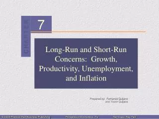
The Short-Run Trade-Off between Inflation and UnemploymentChapter 35
Short-Run Trade-Off between Inflation and Unemployment • Unemployment and Inflation • The natural rate of unemployment depends on various features of the labor market. • Examples include minimum-wage laws, the market power of unions, the role of efficiency wages, and the effectiveness of job search. • The inflation rate depends primarily on growth in the quantity of money, controlled by the Fed.
Short-Run Trade-Off between Inflation and Unemployment • Unemployment and Inflation • Society faces a short-run tradeoff between unemployment and inflation. • If policymakers expand aggregate demand, they can lower unemployment, but only at the cost of higher inflation. • If they contract aggregate demand, they can lower inflation, but at the cost of temporarily higher unemployment.
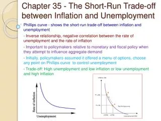
THE PHILLIPS CURVE The Phillips curveshows the short-run trade-off between inflation and unemployment.
B 6 A 2 Phillips curve 4 7 Figure 1 The Phillips Curve Inflation Rate (percent per year) Unemployment 0 Rate (percent)
Aggregate Demand, Aggregate Supply, and the Phillips Curve • The Phillips curve shows the short-run combinations of unemployment and inflation that arise as shifts in the aggregate demand curve move the economy along the short-run aggregate supply curve. • The greater the aggregate demand for goods and services, the greater is the economy’s output, and the higher is the overall price level. • A higher level of output results in a lower level of unemployment.
B 6 B 106 A 102 High A aggregate demand 2 Low aggregate demand 7,500 8,000 4 7 (unemployment (unemployment (output is (output is is 7%) is 4%) 8,000) 7,500) Figure 2 How the Phillips Curve is Related to Aggregate Demand and Aggregate Supply (a) The Model of Aggregate Demand and Aggregate Supply (b) The Phillips Curve Price Inflation Short-run Level Rate aggregate (percent supply per year) Phillips curve Quantity Unemployment 0 0 of Output Rate (percent)
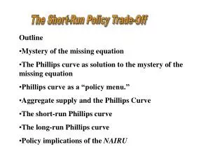
SHIFTS IN THE PHILLIPS CURVE: THE ROLE OF EXPECTATIONS • The Phillips curve seems to offer policymakers a menu of possible inflation and unemployment outcomes.
The Long-Run Phillips Curve • In the 1960s, Friedman and Phelps concluded that inflation and unemployment are unrelated in the long run. • As a result, the long-run Phillips curve is vertical at the natural rate of unemployment. • Monetary policy could be effective in the short run but not in the long run.
B High 1. When the inflation Fed increases the growth rate of the money supply, the 2. . . . but unemployment rate of inflation remains at its natural rate A increases . . . Low in the long run. inflation Figure 3 The Long-Run Phillips Curve Inflation Long-run Rate Phillips curve Unemployment 0 Natural rate of Rate unemployment
3. . . . and 1. An increase in increases the the money supply inflation rate . . . increases aggregate B P2 B demand . . . 2. . . . raises the price level . . . AD2 Figure 4 How the Phillips Curve is Related to Aggregate Demand and Aggregate Supply (a) The Model of Aggregate Demand and Aggregate Supply (b) The Phillips Curve Price Inflation Long-run aggregate Long-run Phillips Level Rate supply curve A P A Aggregate demand, AD Quantity Unemployment 0 Natural rate 0 Natural rate of of Output Rate of output unemployment 4. . . . but leaves output and unemployment at their natural rates.
The Meaning of “Natural” • The “natural” rate of unemployment is the rate to which the economy gravitates in the long run. • The natural rate is not necessarily desirable, nor is it constant over time. • Monetary policy cannot change the natural rate, but other government policies that strengthen labor markets can.
Reconciling Theory and Evidence • Question: How can classical macroeconomic theories predicting a vertical long run Phillips curve be reconciled with the evidence that, in the short run, there is a tradeoff between unemployment and inflation?
The Short-Run Phillips Curve • Expected inflation measures how much people expect the overall price level to change. • In the long run, expected inflation adjusts to changes in actual inflation. • The Fed’s ability to create unexpected inflation exists only in the short run. • Once people anticipate inflation, the only way to get unemployment below the natural rate is for actual inflation to be above the anticipated rate.
The Unemployment Rate = ( ) Expected Actual - Natural ra te of unem ployment - a inflation inflation The Short-Run Phillips Curve • This equation relates the unemployment rate to the natural rate of unemployment, actual inflation, and expected inflation.
2. . . . but in the long run, expected inflation rises, and the short-run Phillips curve shifts to the right. C B Short-run Phillips curve with high expected inflation A 1. Expansionary policy moves the economy up along the short-run Phillips curve . . . Figure 5 How Expected Inflation Shifts the Short-Run Phillips Curve Inflation Long-run Rate Phillips curve Short-run Phillips curve with low expected inflation Unemployment 0 Natural rate of Rate unemployment
The Natural Experiment for the Natural-Rate Hypothesis • The view that unemployment eventually returns to its natural rate, regardless of the rate of inflation, is called the natural-rate hypothesis. • Historical observations support the natural-rate hypothesis. • The concept of a stable Phillips curve broke down in the in the early ’70s. • During the ’70s and ’80s, the economy experienced high inflation and high unemployment simultaneously.
1968 1966 1967 1962 1965 1961 1964 1963 Figure 6 The Phillips Curve in the 1960s Inflation Rate (percent per year) 10 8 6 4 2 0 1 2 3 4 5 6 7 8 9 10 Unemployment Rate (percent)
1973 1971 1969 1970 1968 1972 1966 1967 1962 1965 1961 1964 1963 Figure 7 The Breakdown of the Phillips Curve Inflation Rate (percent per year) 10 8 6 4 2 0 1 2 3 4 5 6 7 8 9 10 Unemployment Rate (percent)
SHIFTS IN THE PHILLIPS CURVE: THE ROLE OF SUPPLY SHOCKS • Historical events have shown that the short-run Phillips curve can shift due to changes in expectations. • The short-run Phillips curve also shifts because of shocks to aggregate supply. • Major adverse changes in aggregate supply can worsen the short-run trade-off between unemployment and inflation. • An adverse supply shock gives policymakers a less favorable trade-off between inflation and unemployment.
SHIFTS IN THE PHILLIPS CURVE: THE ROLE OF SUPPLY SHOCKS • A supply shock is an event that directly alters the firms’ costs, and, as a result, the prices they charge. • This shifts the economy’s aggregate supply curve… • . . . and as a result, the Phillips curve.
4. . . . giving policymakers AS2 a less favorable tradeoff between unemployment and inflation. B P2 B 1. An adverse 3. . . . and shift in aggregate raises supply . . . the price level . . . PC2 Y2 2. . . . lowers output . . . Figure 8 An Adverse Shock to Aggregate Supply (a) The Model of Aggregate Demand and Aggregate Supply (b) The Phillips Curve Price Inflation Level Rate Aggregate supply, AS A A P Aggregate Phillips curve, P C demand Quantity Unemployment 0 0 Y of Output Rate
SHIFTS IN THE PHILLIPS CURVE: THE ROLE OF SUPPLY SHOCKS • In the 1970s, policymakers faced two choices when OPEC cut output and raised worldwide prices of petroleum. • Fight the unemployment battle by expanding aggregate demand and accelerate inflation. • Fight inflation by contracting aggregate demand and endure even higher unemployment.
1981 1975 1980 1974 1979 1978 1977 1976 1973 1972 Figure 9 The Supply Shocks of the 1970s Inflation Rate (percent per year) 10 8 6 4 2 0 1 2 3 4 5 6 7 8 9 10 Unemployment Rate (percent)
THE COST OF REDUCING INFLATION • To reduce inflation, the Fed has to pursue contractionary monetary policy. • When the Fed slows the rate of money growth, it contracts aggregate demand. • This reduces the quantity of goods and services that firms produce. • This leads to a rise in unemployment.
A Short-run Phillips curve with high expected inflation C B Short-run Phillips curve with low expected inflation 2. . . . but in the long run, expected inflation falls, and the short-run Phillips curve shifts to the left. Figure 10 Disinflationary Monetary Policy in the Short Run and the Long Run 1. Contractionary policy moves the economy down along the Inflation short-run Phillips curve . . . Long-run Rate Phillips curve Unemployment 0 Natural rate of Rate unemployment
The Sacrifice Ratio • To reduce inflation, an economy must endure a period of high unemployment and low output. • When the Fed combats inflation, the economy moves down the short-run Phillips curve. • The economy experiences lower inflation but at the cost of higher unemployment.
The Sacrifice Ratio • The sacrifice ratio is the number of percentage points of annual output that is lost in the process of reducing inflation by one percentage point. • An estimate of the sacrifice ratio is five. • To reduce inflation from about 10% to 4% in 1979 would have required an estimated sacrifice of 30% of annual output!
Rational Expectations and the Possibility of Costless Disinflation • The theory of rational expectations suggests that people optimally use all the information they have, including information about government policies, when forecasting the future.
Rational Expectations and the Possibility of Costless Disinflation • Expected inflation explains why there is a trade-off between inflation and unemployment in the short run but not in the long run. • How quickly the short-run trade-off disappears depends on how quickly expectations adjust. • The theory of rational expectations suggests that the sacrifice-ratio could be much smaller than estimated.
The Volcker Disinflation • When Paul Volcker was Fed chairman in the 1970s, inflation was widely viewed as one of the nation’s foremost problems. • Volcker succeeded in reducing inflation (from 10 percent to 4 percent), but at the cost of high unemployment (about 10 percent in 1983).
The Greenspan Era • Alan Greenspan’s term as Fed chairman began with a favorable supply shock. • In 1986, OPEC members abandoned their agreement to restrict supply. • This led to falling inflation and falling unemployment.
1981 1980 A 1979 1982 1984 B 1983 1987 1985 C 1986 Figure 11 The Volcker Disinflation Inflation Rate (percent per year) 10 8 6 4 2 0 1 2 3 4 5 6 7 8 9 10 Unemployment Rate (percent)
1990 1991 1989 1984 1988 1985 1987 2001 1995 1992 2000 1986 1997 1994 1993 1999 2002 1998 1996 Figure 12 The Greenspan Era Inflation Rate (percent per year) 10 8 6 4 2 0 1 2 3 4 5 6 7 8 9 10 Unemployment Rate (percent)
The Greenspan Era • Fluctuations in inflation and unemployment in recent years have been relatively small due to the Fed’s actions.
The Phillips curve describes a negative relationship between inflation and unemployment. • By expanding aggregate demand, policymakers can choose a point on the Phillips curve with higher inflation and lower unemployment.
By contracting aggregate demand, policymakers can choose a point on the Phillips curve with lower inflation and higher unemployment.
The trade-off between inflation and unemployment described by the Phillips curve holds only in the short run. • The long-run Phillips curve is vertical at the natural rate of unemployment.
The short-run Phillips curve also shifts because of shocks to aggregate supply. • An adverse supply shock gives policymakers a less favorable trade-off between inflation and unemployment.
When the Fed contracts growth in the money supply to reduce inflation, it moves the economy along the short-run Phillips curve. • This results in temporarily high unemployment. • The cost of disinflation depends on how quickly expectations of inflation fall.