Download
1 / 27
270 likes | 373 Views
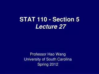
STAT 110 - Section 5 Lecture 23. Professor Hao Wang University of South Carolina Spring 2012. TexPoint fonts used in EMF. Read the TexPoint manual before you delete this box.: A A A A A. Histogram of Mid-Term 2 Grades. min 6 Q1 17 Med:18 Q3 20 Max 24.

E N D
STAT 110 - Section 5 Lecture 23 Professor Hao Wang University of South Carolina Spring 2012 TexPoint fonts used in EMF. Read the TexPoint manual before you delete this box.: AAAAA
Histogram of Mid-Term 2 Grades min 6 Q1 17 Med:18 Q3 20 Max 24
Probability Rules • Any probability is a number between 0 and 1. • So if we observe an event A then we know
Probability Rules • 2. All possible outcomes together must have probability 1. • An outcome must occur on every trial. • The sum of the probabilities for all possible outcomes must be exactly 1.
Probability Rules • The probability that an event does not occur is 1 minus the probability that the event does occur. • This is known as the complement rule. • Suppose that P(A) = .38 • Using this rule we can determine P(not A) • P(not A) = 1- P(A) = 1-.38 = .62 The event “not A” is known as the complement of A which can be written as
Probability Rules • If two events have no outcomes in common, the probability that one or the other occurs is the sum of their individual probabilities. • If this is true then the events are said to be disjoint. Suppose events A and B are disjoint and you know that P(A) = .40 and P(B) = .35. What is the P(A or B)?
Multiplication Rule • Multiplication Rule: If two events are independent then • Independence means that the occurrence of • event A does not affect the occurrence of event B
Probability Models for Sampling sampling distribution – tells what values a statistic takes in repeated samples from the same population and how often it takes those values We can’t predict the outcome of one sample, but the outcomes of many samples have a regular pattern. The distribution of the statistic tells us what values it can take and how often it takes those values
Imagine a biased coin that has a 60% chance of coming up heads. Flip the coin twice. What is the distribution of the percent heads ( ) we see?
Tree diagram What is the distribution of the percent of flips that are heads ( ) ?
What is the distribution of the percent of flips that are heads ( ) ?
What is the distribution of the percent of flips that are heads ( ) ?
So the sampling distribution of is: 0.0 0.5 1.0 P( ) 0.16 0.48 0.36
The sampling distribution of is: 0.0 0.5 1.0 P( ) 0.16 0.48 0.36 So, in this case, even though we’ll usually see 50% or 100% heads, we shouldn’t be surprised to see 0% heads. That still happens 16% of the time. But what if we flipped the coin a lot more?
Imagine a biased coin that has a 60% chance of coming up heads. Flip the coin 1,000 times. What is the distribution of the percent heads ( ) we see?
If we flipped the coin 1,000 times the tree diagram would have 1,000 columns of branches!!!!!!!! Instead we could use the computer to simulate it.
Here are the results of one simulation where the computer repeats the experiment 500 times. On average the percent is close to 0.60, but the spread is pretty small (just between 0.55 and 0.65). And it looks close to normal!
Example on sampling distribution A simple random sample of 501 teens is asked, “Do you approve or disapprove of legal gambling or betting?” Suppose that the true proportion that will say “yes” is .50. The sample proportion who say “Yes” will vary in repeated samples according to a normal distribution with mean 0.5 and standard deviation of about 0.0223.
The sample proportion who say “Yes” will vary in repeated samples according to a normal distribution with mean 0.5 and standard deviation of about 0.022. • What’s the probability that less than .478 say “Yes”? • What’s the probability that .522 or more will say “Yes”? • What’s the probability that 0.60 or more will say “Yes”?
Example on sampling distribution A simple random sample of 1000 college students is taken and asked if they agree that “The dining choices on my campus could be better. If the true percent for the whole population is 60%, the percent in the sample who will say “Yes” should be close to a normal distribution (by the central limit theorem) with mean 0.6 and standard deviation of about 0.0155. Would you be surprised if 65% of the sample said “Yes”?
Would you be surprised if 65% of the sample said “Yes”? That would be surprising, because it should only happen about 6 in 10,000 times!
Example on tree diagram • There is an 80% chance you will make the first red light driving in to work. • If you make the first, there is a 90% chance you will also make the second. • If you miss the first, there is a 90% chance you will also miss the second. • What is the chance you get stopped by both lights? • 0.08 = 8% D) 0.18 = 18% • 0.09 = 9% E) 0.72 = 72% • 0.16 = 16%