Download
1 / 13
140 likes | 530 Views
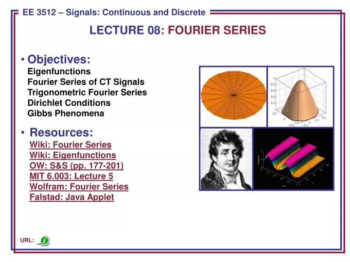
LECTURE 08: FOURIER SERIES. Objectives: Eigenfunctions Fourier Series of CT Signals Trigonometric Fourier Series Dirichlet Conditions Gibbs Phenomena Resources: Wiki: Fourier Series Wiki: Eigenfunctions OW: S&S (pp. 177-201) MIT 6.003: Lecture 5 Wolfram: Fourier Series Falstad : Java Applet.

E N D
LECTURE 08: FOURIER SERIES • Objectives:EigenfunctionsFourier Series of CT SignalsTrigonometric Fourier SeriesDirichlet ConditionsGibbs Phenomena • Resources:Wiki: Fourier SeriesWiki: EigenfunctionsOW: S&S (pp. 177-201)MIT 6.003: Lecture 5Wolfram: Fourier SeriesFalstad: Java Applet URL:
Representation of CT Signals (Again!) • What is an example of a function when applied to an LTI system produces an output that is a scaled version of itself? • The scale factor, k, is referred to as an eigenvalue. The function, k, is referred to as an eigenfunction. • Using the superposition property of LTI systems: • This reduces the problem of finding the response of any LTI system to any signal to the problem of finding the {k}. • What types of things influence the values {k}? We will soon see that the frequency response of this LTI system is one thing that will influence the shape of the output. • We will later generalize this concept of eigenvalues and eigenfunctions to many types of engineering systems and analyses. • The Fourier series is one of many ways to decompose a signal. CT LTI CT LTI
Response of a CT LTI System • Complex exponentials are always eigenfunctions for an LTI system and extremely useful because the output is a scaled version of the input:
(Complex) Fourier Series Representations • What types of signals can be represented as sums of complex exponentials? • CT: s = j (Fourier Transform) signals of the form ejt • DT: z =ej(z-Transform) signals of the form ejn • These representations form the basis of the Fourier Series and Transform. • Consider a periodic signal: • Consider representing a signal as a sum of these exponentials: • Notes: • Periodic with period T • {ck} are the (complex) Fourier series coefficients • k = 0 corresponds to the DC value; k = 1 is the first harmonic; …
Alternate Fourier Series Representations • For real, periodic signals: • These are essentially interchangeable representations. For example, note: • The complex Fourier series is used for most engineering analyses. • How do we compute the Fourier series coefficients? • There are several ways to arrive at the equations for estimating the coefficients. Most are based on concepts of orthogonal functions and vector space projections.
Vector Space Projections • How can we compute the Fourier series coefficients? • One approach is to use the concept of a vector projection: • How do we find the components: • We project the vector onto the correspondingaxis using a dot product. • Note that this works because the three axesare orthogonal: • We can apply the same concept to signals using the notion of a Hilbert space in which each axis represents an eigenfunction (e.g., cos() and sin()):
Computation of the Coefficients • We can make use of the principle of orthogonality in the Hilbert space: • (This can be thought of as an “inner product.”) • We can apply this to our Fourier series: • Using the inner product: • This gives us our Fourier series pair (0=2/T): (synthesis) (analysis)
Convergence of the Fourier Series • How can a series composed of continuous functions (e.g., sines and cosines) approximate a discontinuous function, such as a square wave? • Conditions for which the error in this approximation will tend to zero: • x(t) is absolutely integrableover one period: • In a finite time interval, x(t)has a finite number of maxima and minima. • In a finite time interval, x(t) has a finite number of discontinuities. • These are known as the Dirichlet conditions. They will be satisfied for most signals we encounter in the real world. This implies:
Gibbs Phenomena • Convergence in error can have some interesting characteristics: • This is known as Gibbsphenomena and was firstobserved by Albert Michelsonin 1898. • The Fourier series of a squarewave is plotted as a function ofN, the number of terms in thefinite series. • The limit as N is the averagevalue of x(t) at the discontinuity. • The squared error does converge:
Summary • Introduced the concept of eigenvalues and eigenfunctions. • Developed the concept of a Fourier series. • Discussed three representations of the Fourier series. • Derived an expression for the estimation of the coefficients. • Derived the Fourier series of a periodic pulse train. • Introduced the Dirichlet conditions and Gibbs phenomena. • Discussed convergence properties.
Appendix: Nonlinear Amplifier • Assume we apply a sinewave input to avoltage amplifier under two conditions: • Linear: • In this case, the output is: • The output is a scaled version of the input. • Nonlinear: • Hence, the output signal is at a frequency twice that of the input, which clearly makes this a nonlinear system. • In practice, amplifiers, such as audio power amplifiers, are characterized using a power series: • A single sinewave input generates many frequencies, all harmonically related to the input frequency. This distortion is characterized by figures of merit such as total harmonic distortion and intermodulation. See audio system measurements for more information. Voltage Amplifier vout vin