Download
1 / 38
410 likes | 635 Views
Prerequisites. Almost essential Firm: Basics. The Firm: Optimisation. MICROECONOMICS Principles and Analysis Frank Cowell . Overview. Firm: Optimisation. The setting. Approaches to the firm’s optimisation problem. Stage 1: Cost Minimisation. Stage 2: Profit maximisation.

E N D
Prerequisites Almost essential Firm: Basics The Firm: Optimisation MICROECONOMICS Principles and Analysis Frank Cowell
Overview... Firm: Optimisation The setting Approaches to the firm’s optimisation problem Stage 1: Cost Minimisation Stage 2: Profit maximisation
The optimisation problem • We want to set up and solve a standard optimisation problem • Let's make a quick list of its components • ... and look ahead to the way we will do it for the firm
The optimisation problem • Profit maximisation? • -Technology; other • - 2-stage optimisation • Objectives • Constraints • Method
Construct the objective function • Use the information on prices… • wi • price of input i p • price of output • …and on quantities… • zi • amount of input i q • amount of output How it’s done • …to build the objective function
The firm’s objective function m Swizi i=1 • Cost of inputs: • Summed over all m inputs pq • Revenue: • Subtract Cost from Revenue to get m Swizi i=1 • Profits: pq –
Optimisation: the standard approach • Choose q and z to maximise m Swizi i=1 P := pq – • ...subject to the production constraint... • Could also write this as zZ(q) q £f (z) • ..and some obvious constraints: • You can’t have negative output or negative inputs z³ 0 q³0
A standard optimisation method • If is differentiable… • Set up a Lagrangean to take care of the constraints L(... ) • Write down the First Order Conditions (FOC) necessity ¶ L(... ) = 0 ¶z • Check out second-order conditions sufficiency ¶2 L (... ) ¶z2 • Use FOC to characterise solution z* = …
Uses of FOC • First order conditions are crucial • They are used over and over again in optimisation problems. • For example: • Characterising efficiency. • Analysing “Black box” problems. • Describing the firm's reactions to its environment. • More of that in the next presentation • Right now a word of caution...
A word of warning • We’ve just argued that using FOC is useful. • But sometimes it will yield ambiguous results. • Sometimes it is undefined. • Depends on the shape of the production function f. • You have to check whether it’s appropriate to apply the Lagrangean method • You may need to use other ways of finding an optimum. • Examples coming up…
A way forward • We could just go ahead and solve the maximisation problem • But it makes sense to break it down into two stages • The analysis is a bit easier • You see how to apply optimisation techniques • It gives some important concepts that we can re-use later • First stage is “minimise cost for a given output level” • If you have fixed the output level q… • …then profit max is equivalent to cost min. • Second stage is “find the output level to maximise profits” • Follows the first stage naturally • Uses the results from the first stage. • We deal with stage each in turn
Overview... Firm: Optimisation The setting A fundamental multivariable problem with a brilliant solution Stage 1: Cost Minimisation Stage 2: Profit maximisation
Stage 1 optimisation • Pick a target output level q • Take as given the market prices of inputs w • Maximise profits... • ...by minimising costs m Swi zi i=1
A useful tool • For a given set of input prices w... • …the isocost is the set of points z in input space... • ...that yield a given level of factor cost • These form a hyperplane (straight line)... • ...because of the simple expression for factor-cost structure
z2 z1 Iso-cost lines • Draw set of points where cost of input is c, a constant • Repeat for a higher value of the constant increasing cost • Imposes direction on the diagram... w1z1 + w2z2 = c" w1z1 + w2z2 = c' w1z1 + w2z2 = c Use this to derive optimum
z2 Reducing cost z1 Cost-minimisation • The firm minimises cost... q • Subject to output constraint • Defines the stage 1 problem. • Solution to the problem minimise m Swizi i=1 subject to(z) q z* • But the solution depends on the shape of the input-requirement set Z. • What would happen in other cases?
z2 z1 Convex, but not strictly convex Z Any z in this set is cost-minimising • An interval of solutions
z2 z1 Convex Z, touching axis • Here MRTS21 > w1/ w2at the solution. • Input 2 is “too expensive” and so isn’t used: z2* = 0 z*
z2 z1 Non-convex Z z* • There could be multiple solutions. • But note that there’s no solution point between z* and z** z**
z2 z1 Non-smooth Z MRTS21 is undefined at z*. • z* is unique cost-minimising point for q z* • True for all positive finite values of w1, w2
Cost-minimisation: strictly convex Z • Use the objective function Lagrange multiplier • Minimise • ...and output constraint m Swi zi i=1 • ...to build the Lagrangean + l[q – f(z)] q f (z) • Differentiate w.r.t. z1, ..., zm; set equal to 0 • ... and w.r.t l • Denote cost minimising values by * • Because of strict convexity we have an interior solution • A set of m+1 First-Order Conditions ** ** ** * lf1 (z) = w1 l f2 (z) = w2 … … … lfm(z) = wm one for each input ü ý þ q = (z) output constraint
If isoquants can touch the axes... • Minimise m Swizi i=1 + l [q – f(z)] • Now there is the possibility of corner solutions. • A set of m+1 First-Order Conditions l*f1 (z*) £w1 l*f2 (z*) £w2 … … … l*fm(z*) £wm ü ý þ Interpretation Can get “<” if optimal value of this input is 0 q = f(z*)
From the FOC • If both inputs i and j are used and MRTS is defined then... fi(z*) wi ——— = — fj(z*) wj • MRTS = input price ratio • “implicit” price = market price • If input i could be zero then... fi(z*) wi ——— £ — fj(z*) wj • MRTSji£ input price ratio • “implicit” price £ market price Solution
The solution... • Solving the FOC, you get a cost-minimising value for each input... zi* = Hi(w, q) • ...for the Lagrange multiplier l* = l*(w, q) • ...and for the minimised value of cost itself. • The cost function is defined as C(w, q) := min S wi zi {f(z) ³q} vector of input prices Specified output level
Interpreting the Lagrange multiplier • The solution function: • C(w, q) = Siwizi* • = Siwizi*–l* [f(z*) –q] At the optimum, either the constraint binds or the Lagrange multiplier is zero • Differentiate with respect to q: • Cq(w, q) = SiwiHiq(w, q) • –l* [Si fi(z*)Hiq(w, q) –1] Express demands in terms of (w,q) Vanishes because of FOC l *fi(z*) = wi • Rearrange: • Cq(w, q) = Si [wi– l*fi(z*)] Hiq(w, q) + l* • Cq(w, q) = l* Lagrange multiplier in the stage 1 problem is just marginal cost This result – extremely important in economics – is just an applications of a general “envelope” theorem.
The cost function is an amazingly useful concept • Because it is a solution function... • ...it automatically has very nice properties • These are true for all production functions • And they carry over to applications other than the firm. • We’ll investigate these graphically
C C(w, q+q) ° w1 Properties of C z1* • Draw cost as function of w1 • Cost is non-decreasing in input prices . • Cost is increasing in output. C(w, q) • Cost is concave in input prices. • Shephard’s Lemma C(tw+[1–t]w,q) tC(w,q) + [1–t]C(w,q) C(w,q) ———— = zj* wj
z2 z1 What happens to cost if w changes to tw • Find cost-minimising inputs for w, given q q • Find cost-minimising inputs for tw, given q • So we have: C(tw,q) = i twizi* = t iwizi* = tC(w,q) • z* • z* • The cost function is homogeneous of degree 1 in prices.
Cost Function: 5 things to remember • Non-decreasing in every input price • Increasing in at least one input price • Increasing in output • Concave in prices • Homogeneous of degree 1 in prices • Shephard's Lemma
Example Production function: q z10.1 z20.4 Equivalent form: log q 0.1log z1 + 0.4 log z2 Lagrangean: w1z1 + w2z2 + l [log q – 0.1log z1– 0.4 log z2] FOCs for an interior solution: w1– 0.1 l/ z1= 0 w2– 0.4 l / z2= 0 log q = 0.1log z1 + 0.4 log z2 From the FOCs: log q = 0.1log (0.1 l / w1) + 0.4 log (0.4 l / w2 ) l=0.1–0.2 0.4–0.8w10.2 w20.8 q2 Therefore, from this and the FOCs: w1 z1+ w2 z2 = 0.5 l = 1.649 w10.2 w20.8 q2
Overview... Firm: Optimisation The setting …using the results of stage 1 Stage 1: Cost Minimisation Stage 2: Profit maximisation
Stage 2 optimisation • Take the cost-minimisation problem as solved • Take output price p as given • Use minimised costs C(w,q) • Set up a 1-variable maximisation problem • Choose q to maximise profits • First analyse components of the solution graphically • Tie-in with properties of the firm (in the previous presentation) • Then we come back to the formal solution
Average and marginal cost increasing returns to scale decreasing returns to scale • The average cost curve p • Slope of AC depends on RTS • Marginal cost cuts AC at its minimum Cq C/q q q
q q q q q q* Revenue and profits • A given market price p • Revenue if output is q • Cost if output is q • Profits if output is q • Profits vary with q • Maximum profits Cq C/q p P • price = marginal cost q
What happens if price is low... Cq C/q p • price < marginal cost q* = 0 q
Profit maximisation • Objective is to choose q to max: pq –C (w, q) “Revenue minus minimised cost” • From the First-Order Conditions if q* > 0: p = Cq(w, q*) C(w, q*) p ³ ———— q* “Price equals marginal cost” “Price covers average cost” • In general: covers both the cases: q* > 0 and q* = 0 p £Cq(w, q*) pq* ³ C(w, q*)
Example (continued) Production function: q z10.1 z20.4 Resulting cost function: C(w, q) = 1.649 w10.2 w20.8 q2 Profits: pq – C(w, q) = pq – A q2 where A:= 1.649 w10.2 w20.8 FOC: p – 2 Aq = 0 Result: q = p / 2A = 0.3031 w1–0.2 w2–0.8 p
Summary • Key point: Profit maximisation can be viewed in two stages: • Stage 1: choose inputs to minimise cost • Stage 2: choose output to maximise profit • What next? Use these to predict firm's reactions Review Review