Download
1 / 26
260 likes | 422 Views
NOAA Earth System Research Laboratory. Review of “Covariance Localization” in Ensemble Filters. Tom Hamill NOAA Earth System Research Lab, Boulder, CO tom.hamill@noaa.gov. Canonical ensemble Kalman filter update equations. H = (possibly nonlinear) operator from model to

E N D
NOAA Earth System Research Laboratory Review of “Covariance Localization” in Ensemble Filters Tom Hamill NOAA Earth System Research Lab, Boulder, CO tom.hamill@noaa.gov
Canonical ensemble Kalman filter update equations H= (possibly nonlinear) operator from model to observation space x = state vector (ifor ith member ) Notes: • An ensemble of parallel data assimilation cycles is conducted, here assimilating perturbed observations . • Background-error covariances are estimated using the ensemble.
Example of covariance localization obs location Background-error correlations estimated from 25 members of a 200-member ensemble exhibit a large amount of structure that does not appear to have any physical meaning. Without correction, an observation at the dotted location would produce increments across the globe. Proposed solution is element-wise multiplication of the ensemble estimates (a) with a smooth correlation function (c) to produce (d), which now resembles the large-ensemble estimate (b). This has been dubbed “covariance localization.” from Hamill, Chapter 6 of “Predictability of Weather and Climate”
How covariance localization is commonly implemented in EnKF sis typically a compactly supported function similar in shape to a Gaussian, 1.0 at observation location. See Gaspari and Cohn, 1999, QJRMS, 125, 723-757, eq. 4.10
Why localization ? Relative sampling error’s dependence on ensemble size, correlation. True background-error covariance of model with two grid points: and obs at grid point 1 with error covariance Suppose there is inaccurate estimate of background-error covariance matrix How do errors change with correlation and ensemble size? Relative error is large when correlation and/or ensemble size is small. Ref: Hamill et al, 2001, MWR, 129, pp. 2776-2790
Spreads and errors as function of localization length scale (1) Small ensembles minimize error with short length scale, large ensemble with longer length scale. That is, less localization needed for large ensemble. (2) The longer the localization length scale, the less spread in the posterior ensemble. Ref: Houtekamer and Mitchell, 2001, MWR, 129, pp 123-137.
Localization adds effective degrees of freedom to background-error covariance model • Experiments with toy 2-layer primitive equation model • With few members, eigenvalue spectrum of background error covariance is very steep, and with n-member ensemble, only n-1 degrees of freedom; with more members, less steep spectrum. • Covariance localization in ensemble increases the effective degrees of freedom, makes eigenvalue spectrum flatter; more ways the ensemble can adjust to the data. • At the end of the data assimilation, though, you still have posterior ensemble with only n-1 degrees of freedom. Ref: Hamill et al, 2001, MWR, 129, pp. 2776-2790
Increasing localization scale increases CPU run time • Ensemble filters commonly serially process the observations. + + + + + + + + + + + + + + + + + + + + + + + + + + + + + + + + + + + + + + + + + + + + + + + + + + + + + + + + + + + + + + + + + + + + + + + + + + + + + + + + + + + + + + + + + + + + + + + + + + + + + + + + + + + + + + + + + + + + + + + + + + + + + + + + + + + + + + + + + + + + + + + + + + + + + + + + + + + + + + + + + + + + + + + + + + + + + + + + + + + + + + + + + + + + + + + + + + + + + + + + + + + + + + + + + + + + + + + + + + + + + + + + + + + + + + + + + + + + + + + + + + + + + + + + + + + + + + + + + + + + + + + + + + + + + + + + + + + + + + + + + + + + + + + + + + + + + + + + + + + + + + + + + + + + + + + + + + + + + + + + + + + + + + + + + + + + + + + + + + + + + + + + + + + + + + + + + + + + + + + + + + + + + + + + + + + + + + + + + + + + + + + + + + + + + + + + + + + + + + + + + + + + + + + + + + + + + + + + + + + + + + + + + + + + + + + + + + + + + + + + + + + + + + + + + + + + + + + + + + + + + + + + + + + + + signs are grid points. Red dot: observation location. Blue disc: area spanned by localization function. Dashed line: box enclosing all possible grid points that must be updated given this localization scale.
Covariance localization introduces imbalances • Scaled imbalance (imbalance / increment magnitude) for 3 gravest vertical modes, pair of 32- member ensembles. • Imbalance measured by comparing digitally filtered state to unfiltered. • Larger scaled imbalance at shorter correlation length scales. • The imbalance may limit the growth of spread, making background-error covariance model estimated from ensemble less accurate. Ref: Mitchell and Houtekamer, 2002, MWR, 130, pp. 2791-2808. See also J. Kepert’s talk and A. Lorenc, 2003, QJRMS, 129, 3183-3203.
Synthesis “Localization scale is a tuning parameter that trades off computational effort, sampling error, and imbalance error.” (Ref: Zhou et al., 2008, MWR, 136, 678-698.)
Localization by inversely scaling observation-error covariances 1.0 s 0.0 x1 x2 x3 obs at x2, H=I, variance R something akin to covariance localization can be obtained by inversely scaling the observation-error variance rather than modifying the background-error covariances. Pioneered in LETKF. Ref: Hunt et al. 2007, Physica D, 230, 112-126.
“Hierarchical” ensemble filter • Suppose m groups of n-member ensembles. Then m estimates of background-error covariance relationships between obs location, model grid point (*). • Kalman filter update: effectively a linear regression analysis, compute increment in state variable x, given increments for observation variable, yo. Hence m sample values of (i.e., K(*)) are available. • Assume correct is a random draw from same distribution the m samples drawn from. • “Regression confidence factor” chosen to minimize • An “on-the-fly” moderation of covariances; replace with . Ref: Jeff Anderson, 2007, Physica D, 230, 99-111.
Anderson’s hierarchicalensemble filter (continued) Regression confidence factor. Hovmoller of regression confidence factor for Lorenz ‘96 model assimilations for observations at red line, 16-group ensemble, 14 members. min 0 when spread of is large relative to mean. min 1 when spread is small relative to mean. Is the variability with time a feature or a bug?
Example of where regressionconfidence factor may induce unrealistic increments White lines: background sea-level pressure. Colors: background precipitable water. Observation 1 hPa less than background at dot. Red contours: precipitable water analysis increment due to SLP observation, dashed is negative. Uses Gaspari-Cohn localization here.
Example of where regressionconfidence factor may induce unrealistic increments Imagine gain calculation along black line, and how it may vary if several parallel ensemble filters were run.
Gain calculations along cross-section Here, the spread in gains is small relative to the magnitude of gain; hence 1 K (Gain) 0 Distance, left to right
Gain calculationsalong cross-section Here, the spread in gains is large relative to the magnitude of gain; hence 0 K (Gain) 0 Distance, left to right
Gain calculationsalong cross-section Here, the spread in gains is large relative to the magnitude of gain; hence 0 Regression Confidence Factor 1 K (Gain) 0 0 Distance, left to right Distance, left to right
Gain calculationsalong cross-section The product of & K now produces a larger region in the middle with nearly zero gain, and hence near-zero increment. This may be, in some circumstances, non-physical. K (Gain) 0 Distance, left to right
Other localization ideas • Multiscale filter: replaces at each update time, the sample covariance with a multiscale tree, composed of nodes distributed over a relatively small number of discrete scales • Ref: Zhou et al. 2008, MWR, 136, 678-698.
Other localization ideas • Spectral localization: Filter covariances after transformation to spectral space, or combine spectral and grid-point localization. • Ref: Buehner and Charron, 2007, QJRMS, 133, 615-630.
“Successive Covariance Localization”Fuqing Zhang, Penn State • Adjust ensemble to regular network of observations using a broad localization length scale. • Where observations are sparse, use of short localization length scale will result in imbalances, “holes” in analysis-error spread, increased analysis errors. • Adjust modified ensemble further to high-density observations using a short localization length scale. • Where dense observations, use of long localization length scale will smooth out mesoscale detail, trust ensemble covariance model too much, and strip too much variance from ensemble. • Effective compromise that works across both data-dense and data-sparse regions?
Change model variables? • Localization in (z, , ) (streamfunction, velocity potential) instead of (z, u, v)? • Ref: J. Kepert, 2006, tinyurl.com/4j539t • Figure to right: errors for normal localization, localization in (z, , ) space, and localization zeroing out (z- ) & (-)
Ensemble Correlations Raised to a Power (ECO-RAP) • Craig Bishop will present this idea in more detail in the next talk.
Conclusions • Some form of covariance localization is a practical necessity for EnKF NWP applications. • Because of drawbacks (e.g., imbalances introduced), active search for improved localization algorithms. • Many interesting alternatives, but community not yet united behind one obviously superior approach. Alternatives tend to have their own set of strengths and weaknesses.