Download
1 / 31
310 likes | 311 Views
Searching and Binary Search Trees. CSCI 3333 Data Structures. Acknowledgement. Dr. Yue Mr. Charles Moen Dr. Wei Ding Ms. Krishani Abeysekera Dr. Michael Goodrich Dr. Richard F. Gilberg. Searching. Google: era of searching! Many type of searching: Search engines: best match.

E N D
Searching andBinary Search Trees CSCI 3333 Data Structures
Acknowledgement • Dr. Yue • Mr. Charles Moen • Dr. Wei Ding • Ms. Krishani Abeysekera • Dr. Michael Goodrich • Dr. Richard F. Gilberg
Searching • Google: era of searching! • Many type of searching: • Search engines: best match. • Key searching: searching for records with specified key values. • Keys are usually assumed to come from a total order (e.g. integers or strings) • Keys are usually assumed to be unique. No two records have the same key.
Naïve Linear Search Algorithm LinearSearch(r, key) Input: r: an array of record. Each record contains a unique key. key: key to be found. Output: i: the index such that r[i] contains the key, or -1 if not found. foreach element in r with index i if r[i].key = key return i; end foreach return -1
Naïve Linear Search • Linear time in finding! • Only suitable when n is very small. • No ‘pre-processing’.
Binary Search • Assume the array has already been sorted in ascending key value. • Example: find(7) 0 1 3 4 5 7 8 9 11 14 16 18 19 m h l 0 1 3 4 5 7 8 9 11 14 16 18 19 m h l 0 1 3 4 5 7 8 9 11 14 16 18 19 m h l 0 1 3 4 5 7 8 9 11 14 16 18 19 l=m =h
Binary Search Algorithm Algorithm BinarySearch(r, key) Input: r: an array of record sorted by its key values. Each record contains a unique key. key: key to be found. Output: i: the index such that r[i] contains the key, or -1 if not found. low = 0; high = r.size – 1 while (low <= high) do mid = (high – low) / 2 if r[mid].key > key then high = mid-1 if r[mid].key = key then return mid; if r[mid].key < key then low = mid + 1 end while return -1;
Binary Search • O(lg n) in finding! • Especially suitable for relatively static sets of records. • Question: can we find a searching algorithm of O(1)? • Question: can we find a searching algorithm of O(lg N), where the time complexity for insert and delete is better? • Average case • Worst case
Binary Search Trees • A binary search tree (BST) is a binary tree which has the following properties: • Each node has a unique key value. • The left subtree of a node contains only values less than the node's value. • The right subtree of a node contains only key values greater than the node's value. • Each subtree is itself a binary search tree.
BST • An inorder traversal of a binary search trees visits the keys in increasing order. • Note that there are variations in the formulation of BST. The one defined in the textbook is somewhat different and is best mapped to implement a dictionary. • Duplicate key values allowed. • Records stored in leaf nodes. • Leaf nodes store no key. • The version of BST used here is more basic, easier to understand, and more popular.
Searching a BST • Similar to binary search. • Each key comparison with a node will result in one of these: • target < node key => search left subtree. • target = node key => found! • target > node key => search right subtree. • Difference with binary search: do not always eliminate about half of the candidates. • The BST may not be balanced.
BST Find Algorithm (Recursive) Algorithm Find(r, target) Input: r: root of a BST. target: key to be found. Output: p: the node in the BST that contains the target; null if not found. if r = null return null; if target = r.key return r; if target < r.key return find(r.leftChild(),target) else // target > r.key return find(r.rightChild(),target) end if
BST Find Algorithm (Iterative) Algorithm Find(r, target) Input: r: root of a BST. target: key to be found. Output: p: the node in the BST that contains the target; null if not found. result = r while result != null do if target = result.key return result; if target < result.key then result = result.leftChild() else // target > r.key result = result.rightChild() end if end while return result
Time Complexity • Depend on the shape of the BST. • Worst case: O(n) for unbalanced trees. • Average case: O(lg N)
BST Insert • Insert a record rec with key rec.key. • Idea: search for rec.key in the BST. • If found => error (keys are supposed to be unique) • If not found => ready to insert (however, need to remember the parent node for insertion).
BST Insert Algorithm (Iterative) Algorithm Insert(r, rec) Input: r: root of a BST. rec: record to be found. Output: whether the insertion is successful. Side Effect: r may be updated. curr = r parent = null // find the location for insertion. while (curr != null) do if curr.key = rec.key then return false // duplicate key: unsuccessful insertion else if rec.key < curr.key then curr = curr.leftChild() parent = curr else // rec.key > curr.key curr = curr.rightChild() parent = curr end if end while
BST Insert (Continue) // create new node for inserrtion newNode = new Node(rec) newNode.parent = parent // Insertion. if parent = null then r = newNode; else if rec.key < parent.key then parent.leftChild = newNode else parent.rightChild = newNode end if return true
BST Delete • More complicated • Cannot delete a parent without arranging for the children! • Who take care of the children? Grandparent. • If there is no grandparent? The root is deleted and a child will become the root. • Need to keep track of the parent of the node to be deleted.
BST Delete • Find the node with the key to be deleted. • If not found, deletion is not successful. • Deletion of the node p: • No child: simple deletion • Single child: connect the parent of p to the single child of p. • Both children: • Connect the parent of p to the right child of p. • Connect the left child of p as the left child of the immediate successor of p.
BST Delete Algorithm Algorithm Delete(r, target) Input: r: root of a BST. target: key of the record to be found. Output: whether the deletion is successful. Side Effect: r is updated if the root node is deleted. curr = r; parent = null // find the location for insertion. while (curr != null and curr.key != target) do if target < curr.key then curr = curr.left parent = curr else // target > curr.key curr = curr.right parent = curr end if end while
BST Delete Algorithm (Continue) if curr = null then return false; // not found end if if curr.right = null then // no right child if parent = null then // root deleted r = r.left else if target < parent.key then parent.left = curr.left else parent.right = curr.left end if end if else
BST Delete Algorithm (Continue) // has right child if curr.left = null then // has a right child but no left child if parent = null then // root deleted r = r.right else if target < parent.key then parent.left = curr.right else parent.right = curr.right end if end if else
BST Delete Algorithm (Continue) // has both left and right children // find immediate successor. immedSucc = curr.right while (immedSucc.left != null) immedSucc = immedSucc.left end while immedSucc.left = curr.left
BST Delete Algorithm (Continue) if parent = null then // root deleted r = r.right else if target < parent.key then parent.left = curr.right else parent.right = curr.right end if end if end if delete curr end if
Time Complexity • Worst case: O(N) • Result in unbalanced tree.
Unbalanced BST • Two approaches: • Reorganization when the trees become very unbalanced. • Use balanced BST • Balanced BST • Many potential definitions. • Height = O(lg n)