Download
1 / 14
140 likes | 143 Views
This algorithm combines ideas from variational data assimilation, iterated Kalman filters, and ensemble transform Kalman filters to estimate model error and assimilate data. It can calculate optimal estimates of model state variables, empirical parameters, and model error, as well as uncertainty and information content of observations.

E N D
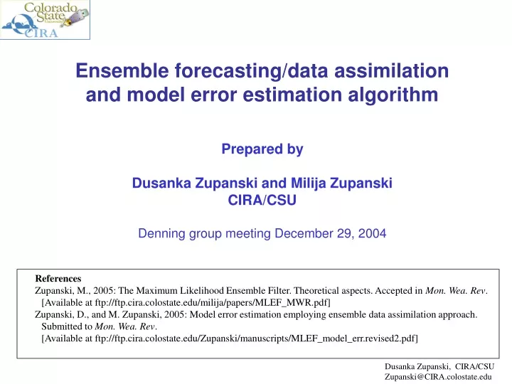
Ensemble forecasting/data assimilation and model error estimation algorithm Prepared by Dusanka Zupanski and Milija Zupanski CIRA/CSU Denning group meeting December 29, 2004 References Zupanski, M., 2005: The Maximum Likelihood Ensemble Filter. Theoretical aspects. Accepted in Mon. Wea. Rev. [Available at ftp://ftp.cira.colostate.edu/milija/papers/MLEF_MWR.pdf] Zupanski, D., and M. Zupanski, 2005: Model error estimation employing ensemble data assimilation approach. Submitted to Mon. Wea. Rev. [Available at ftp://ftp.cira.colostate.edu/Zupanski/manuscripts/MLEF_model_err.revised2.pdf] Dusanka Zupanski, CIRA/CSU Zupanski@CIRA.colostate.edu
Maximum Likelihood Ensemble Filter (MLEF) • Developed using ideas from: • Variational data assimilation(3DVAR, 4DVAR) • Iterated Kalman Filters • Ensemble Transform Kalman Filter (ETKF, Bishop et al. 2001) What the MLEF can do? • Calculate optimal estimatesof: - model state variables (e.g., carbon fluxes, sources, sinks) - empirical parameters (e.g., light response, allocation, drought stress) - model error (bias) - boundary conditions error (lateral, top, bottom boundaries) • Calculate uncertainty of all estimates • Calculate information content of observations (observability in ensemble subspace) Dusanka Zupanski, CIRA/CSU Zupanski@CIRA.colostate.edu
What the MLEF can do (continued)? • Calculate sensitivity, defined in calculus of variations - find the most likely sources/sinks of carbon • Define targeted observations strategies, based on the forecast uncertainty - the system knows where, when and which observations are needed in order to reduce forecast uncertainty • Acquire new knowledge about atmospheric and carbon processes - the system learns from the past about the state variables, model errors, empirical parameters, etc. - the system is adaptive (updates error covariance matrices in each data assimilation cycle) Dusanka Zupanski, CIRA/CSU Zupanski@CIRA.colostate.edu
DATA ASSIMILATION (ESTIMATION THEORY) Discrete stochastic-dynamic model Gurney et al. (2003, Tellus) (?) xk-1 – model state wk-1 – model error (stochastic forcing) M – non-linear dynamic (NWP) model G – operator reflecting the state dependence of model error Discrete stochastic observation model Gurney et al. (2003, Tellus) ek – measurement + representativeness error H – non-linear observation operator (M D ) Dusanka Zupanski, CIRA/CSU Zupanski@CIRA.colostate.edu
MLEF APPROACH Minimize cost function J Change of variable - model state vector of dim Nstate >>Nens - control vector in ensemble space of dim Nens Dusanka Zupanski, CIRA/CSU Zupanski@CIRA.colostate.edu
MLEF APPROACH (continued) Analysis error covariance In Gurney et al. (2003) Dusanka Zupanski, CIRA/CSU Zupanski@CIRA.colostate.edu
MLEF APPROACH (continued) Forecast error covariance In standard Kalman filter Dusanka Zupanski, CIRA/CSU Zupanski@CIRA.colostate.edu
MLEF application to calculate information content RAMS model example Observation categories within the same cycle Multiple cycles Initial cycles carry more information. Model has a capability to learn from the observations in later cycles. Dusanka Zupanski, CIRA/CSU Zupanski@CIRA.colostate.edu
Ensemble Data Assimilation results with CSU global shallow-water model Observation categories within the same cycle Multiple cycles Impact (contribution) from each observation type can be quantified ! Milija Zupanski, CIRA/CSU ZupanskiM@CIRA.colostate.edu
MLEF Algorithm prep_ensda.sh WARM start: Copy files from previously completed cycle COLD start: Run randomly-perturbed ensemble forecasts to initialize fcst err cov cycle_ensda.sh icycle < N_cycles_max fcsterr_cov.sh - Prepare first-guess (background) vector - Prepare forecast error covariance (from ensembles) prep_obs.sh Given ‘OBSTYPE’ and ‘delobs’, select and copy available obs files assimilation.sh Iterative minimization of cost function, save current cycle output Dusanka Zupanski, CIRA/CSU Zupanski@CIRA.colostate.edu
MLEF Algorithm assimilation.sh script assimilation.sh iter < ioutmax forward.sh: Transformation from model space to observation space Hessian preconditioning (only for iter=1) Gradient calculation (ensembles) Cost function calculation (diagnostic) Minimization (ensemble subspace) Step-length (line-search) Control variable update (transformation from ensemble subspace to model (physical) space) - Analysis error covariance calculation - Save current cycle output files - Post-processing (chi-square, RMS, etc.) Dusanka Zupanski, CIRA/CSU Zupanski@CIRA.colostate.edu
MLEF Algorithm Options Models: KdVB, GEOS, SWM, RAMS, … Observations: Synthetic or include various real observations Obs. operators: Include various forward operators Solution Type: Mode (max likelihood-MLEF) or Mean (ensemble mean ETKF) Estimator: Filter or Smoother Control variable: Initial conditions, Model bias, Model parameters Covariances: Localized, or Non-localized forecast error covariance Minimization: Minimization algorithm (C-G, L-BFGS) MPI: ParallelMPI run or a Single processor run Verifications: Innovation statistics (chi-square test, K-S test), RMS-errors Dusanka Zupanski, CIRA/CSU Zupanski@CIRA.colostate.edu
Tasks • Decide which MODELs will be used (LPDM, SiB-CASA-RAMS, PCTM) • In initial experiments use MODEL as in Gurney et al. (2003) • Install LAPACK on your computer, unless it already exists. Compile with 32 bit object code option (LAPACK can be found at http://www.cs.colorado.edu/~lapack) • Install MLEF algorithm on your computer • Include MODEL into MLEF • - develop an interface between MODEL and MLEF • (a template from SWM, RAMS is available) • - prepare all input files for the model • Prepare observations - synthetic observations of atmospheric and carbon variables - separate observations into groups (if needed) - define data assimilation interval Dusanka Zupanski, CIRA/CSU Zupanski@CIRA.colostate.edu
Tasks (continued) • Perform initial data assimilation experiments with synthetic observations - perfect model assumption experiments - parameter estimation experiments - model error estimation experiments • Develop observation operators for: - atmospheric observations (u,v,T,p,q, etc.) - carbon observations • Data assimilation and ensemble forecasting experiments with real observations - LPDM - SiB-CASA-RAMS - PCTM Major development assignments • Model related tasks (LPDM, SiB-CASA-RAMS, PCTM) • Observation operators related tasks Dusanka Zupanski, CIRA/CSU Zupanski@CIRA.colostate.edu