Download
1 / 61
770 likes | 1.11k Views
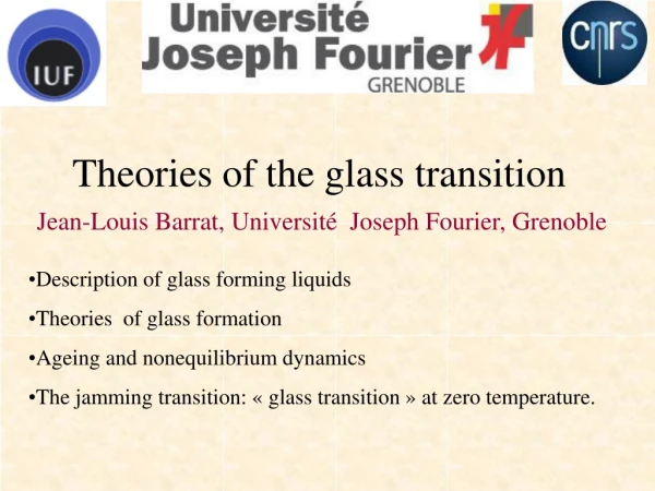
Theories of the glass transition. Jean-Louis Barrat, Université Joseph Fourier, Grenoble . Description of glass forming liquids Theories of glass formation Ageing and nonequilibrium dynamics The jamming transition: « glass transition » at zero temperature.

E N D
Theories of the glass transition Jean-Louis Barrat, Université Joseph Fourier, Grenoble • Description of glass forming liquids • Theories of glass formation • Ageing and nonequilibrium dynamics • The jamming transition: « glass transition » at zero temperature.
http://en.wikipedia.org/wiki/Phase_transition The liquid-glass transition is observed in many polymers and other liquids that can be supercooled far below the melting point of the crystalline phase. It is not a transition between thermodynamic ground states. Glass is a quenched disorder state, and its entropy, density, and so on, depend on the thermal history. Therefore, the glass transition is primarily a dynamic phenomenon: on cooling a liquid, internal degrees of freedom successively fall out of equilibrium. Some theoretical methods predict an underlying phase transition in the hypothetical limit of infinitely long relaxation times. No direct experimental evidence supports the existence of these transitions.
Definition of a glass ? Time scale separation between microscopic, experimental, relaxation; the system is out of equilibrium on the experimental time scale. (cf. S.K. Ma, Statistical Physics)
- « hard » glasses:(SiO2, bulk metallic glasses) Large shear modulus (Gpa) ; spectroscopy, X-ray and neutron scattering, calorimetry - «soft » glasses : Colloids, foams, granular systems.. Small elastic modulus (Mpa). Rheology, light scattering -other examples:vortex glasses , spin glasses Metallic glass under strain Colloidal glass
Glass transition defined by typical viscosity (or relaxation time t) of 1013 Poise. Arbitrary but convenient Water= 0.01 Honey= 100 Arrhenius plot: log(time) or log(viscosity) versus 1/T. Similar behaviour for relaxation times obtained using different methods (dielectric relaxation, NMR) . a relaxation time ta
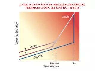
Angell’s classification: « strong » and « fragile » glasses • (T) defines Tg: (Tg) = 1013 Poise (arbitrary definition) • N.B.: 1013P corresponds to alpha relaxation time of 100 seconds • log() vs Tg/T : quantifies deviations from Arrhenius behaviour Angell-plot (Uhlmann)
Strong curvature: ‘fragile’ glass. Organic (OTP: Orthoterphenyl), ionic (CKN: CaK NO3) ; Energy barrier increases as T decreases, cooperative aspects. Weak curvature : ‘strong’ glass .covalent bonding, SiO2, ZnCl2, BeF2
What about the microscopic structure ? Not much happens… S(q) = N-1kj exp(i q (rk – rj)) Hard to see a « critical phenomenon » - or perhaps not the right order parameter.
Time dependent correlations: microscopic dynamics A(t), B(t) observables (density fluctuation , moment dipole moment) AB(t,t’) = A(t) B(t’) AB(t,t’) = A(t) B(t’) = A(t-t’) B(0) = AB(t-t’)
Transformation to frequency domain ’’(): imaginary part of FT((t)) ’’():imaginary part of the susceptibility ’’() = /(kBT) ’’()
Example:dielectric relaxation Lunkenheimer et al. (2001)
Summary • strong slowing down (temperature, pressure,…) • transition to a nonergodic ‘phase’ • increase of the apparent free energy barriers with decreasing T • no long range order • no obvious length scale • complex time dependent relaxation • stretched alpha relaxation (Non Debye) • thermodynamic “anomalies” associated with glass “transition” at low temperature : ageing
Theories of glass formation • Adams-Gibbs approach and random first order theory • Mode-coupling theories: dynamical phase transition • P-spin mean field models – a unified view. • Kinetically frustrated models • Frustrated domain growth
« Entropic » theories, Adams Gibbs (1965), RFOT (1985) Energy (free energy ?) landscape Configuration entropy = log(number of minima with energy u ) Vibrational free energy of the minimum at energy u
Assume independent of u Minima occupied at temperature verify Problem if sc(u) vanishes at umin with a finite slope Equilibrium impossible at temperatures below T0 « Entropic crisis »
Calculating sc(u) is the difficult part but has been done using various approximations (Mézard-Parisi, Kirpatrick-Wolynes, replica approach) ; these schemes confirm the existence of an ‘entropic crisis’ at a finite temperature. In the replica scheme, the order parameter is the correlation between two replica of the system coupled by a vanishingly small potential (symmetry breaking field). Below T0, all replica in the same state, configurational entropy vanishes. (See Mézard and Parisi, J. Chem. Phys. 1999)
Cpnnection to dynamics: Adams Gibbs 1965 (See Bouchaud Biroli cond-mat/0406317 for modern variants) - Nd independent ‘cooperative rearranging regions’ (CRR) . -Number of atoms within one region= N/Nd = z -Configuration entropy sc= Nd k/V -Time scale for a re-arrangement = t0 exp( +zd/kBT) A= Nd/ V Correlation well verified in simulation and experiment
Mode coupling approaches Simplified mode coupling (Gezti 1984)
Finally: Combine with Stokes Einstein « viscosity feedback » ; divergence at a finite value of the control parameter T (or pressure or density). Dynamical phase transition.
More technical approaches -projection operators (Götze) - Self consistent one loop approximation in perturbation theory (Mazenko) Eventually, closed equations for correlation functions: V(q,q’) dependent on liquid structure factor S(q), hence on temperature and density
Simplified model, S(q) = (q-q0): Laplace transform Look for nonergodic behaviour non ergodic solution if l2 > l2c =4
Nonlinear differential equation with memory term. Sophisticated analysis possible close to the « critical point » l2 = l2c =4 (Götze). for l2 = l2c =4 we have With l= 1/2
Solution: Correlation function approaches a plateau with a power law, nonuniversal exponent a. Multiple time scale analysis, different time scales depend on the distance from critical point e=l2 - l2c .
Generic properties of solutions • Numerical solution, hard spheres • Temperature (density) Tc at which the relaxation time diverges • Close to Tc relaxation time diverges as (T-Tc)-
Generic properties – approach to the plateau ( relaxation) – time scale • Near the plateau • B/z + zG(z)2 - LT[G(t)2](z) = 0 • B and can be computed from the full equations. • Near the plateau, factorization property • Short times G(x) x-a • Long times G(x) xb (von Schweidler) • a, b , vérify • (1-a)2/(1-2a)=(1+b)2/(1+2b) = • exponent of (T-Tc)- verifies = 1/2a + 1/2b
Generic properties – terminal relaxation (a) – Time scale • Shape of the curve independent of T during relaxation for T > Tc; “time-temperature superposition principle” • Good approximation Kohlrausch-Williams-Watts (streteched exponential) • (t) = A exp(- (t/)) • N.B. not an exact solution! • For T < Tc, f (plateau value) increases as (Tc – T)1/2
Comparison with experiments/simulation: • Tc does not exist in practice • Numerical predictions for Tc are above Tg • Good description for the first stages of slowing down (typically relaxation times up to 10-8 s ) , Probably better for colloids • Predictive theory: « reentrant » glass transition for attractive colloidal systems
Reentrant glass transition in attractive colloids Theory Experiment
‘p-spin’ models in mean field – A unified approach ? p=3 Jijkrandom variable with variance « mean field » limit (infinite N) ‘Mode coupling approximation’ becomes exact
Model has -dynamical transition at Td ;described by nonlinear equations of MCT in liquids. Appearance of many minima in free energy landscape, separated by infinite barriers (mean field). - Static transition of Adams-Gibbs type (entropy vanishes with finite slope) at TK Both aspects come from the mean field limit, but probably something remains in finite dimensions... (Mézard –Parisi)
Kinetically frustrated spin models Introduced by Fredrickson and Andersen in 1984. Many similar models, for a review see General idea: at low T weak concentration of mobile regions. To allow structural relaxation these mobile regions must explore the volume, and this takes time
Fredrickson-Andersen: spins ni=0,1 onlattice. No interactions, trivial Hamiltonian ni =1 mobile ni=0 frozen Rule of the game : evolution 1->0 or 0->1 possible only if spin i has at least one mobile neighbor. Transition rates verify detailed balance At equilibrium concentration of mobile zones :
At low T, relaxation proceeds through diffusion of isolated mobile zones. diffusion coefficient of a zone: D= exp(-1/T) Distance between mobile zones : 1/c (en d=1) Relaxation time: D x (1/c)2
East : spins ni=0,1 No interactions, trivial Hamiltonian ni =1 mobile ; ni=0 frozen Rule of the game : evolution 1->0 ou 0->1 possible only if spin i a has its left neighnour mobile. Transition rates verify detailed balance At equilibrium mobile zones concentration:
Fragile behaviour 100000..0001 domain of length d=2k n(k) = number of spins to relax the one on the right n(k) = n(k-1) +1 = k+1 Time t(d) = exp(n(k)/T) = exp( ln(d)/ T ln(2)) Using d=1/c = exp(1/T) one gets the result Results can be modified by adjusting the rules of the game…
Models explain dynamical heterogeneities in terms of space/time correlations non constrained FA East Static configurations are the same in all three cases!
-Highlights the importance of dynamical heterogeneities -Phase transition in the space of trajectories, with a critical point at T=0 (Garrahan, van Wijland) Dynamical heterogeneities Displacement of particules over a time interval 50ta Can also be characterized in experiments (confocal microscopy, hole burning)
Notion of cooperativity: Xi (t) = di(t)- <di(t)> where di(t) is the displacement of particle i in the interval [0,t]. The idea (Heuer and Doliwa, PRE 2000) is to compare the fluctuations at the one particle level and over the whole system: Cooperativity goes trough a maximum at t*
Approach can be generalized to any observable mobility field « 4-point susceptibility » Relates to the correlation volume at time t, and is also the variance of the global correlation: where
Hypothesis: system approaches spinodal instability, but domain growth limited by frustration Possible realizations: -icosaedral order preferred locally, frustrated in 3d. -magnetic system with ferromagnetic interactions at long range, antiferro or dipolar at long range Frustration limits domain growth to a size R
Refinments with size distribution, translation-rotation decoupling, etc… See
A small problem… Minimal models for FLD model (Reichman et Geissler, Phys. Rev. E. 2003) Formation of a lamellar phase and associated critical dynamics (bloc copolymers, magnetic layers), rather different from glassy dynamics
Some conclusions… • « THE » theory does not exist • Many different and complementary approaches. Models can capture some aspects of real systems, but also miss many – risk of studying model artefacts. • NB: not mentioned: free volume (recent version by D. Long and F. Lequeux), trap models, lattice gas models....
http://www.theory.com Retail stores in Aspen, New-York, Paris, London, Tokyo, Beijing… THEORY return and exchange policy: We want you to be completely satisfied with your Theory purchase. We will happily accept your return or exchange of product in original condition with all tags attached when accompanied by a receipt within 14 days of purchase at any Theory retail store.
Inside the glassy state: nonequilibrium relaxation (ageing) http://en.wikipedia.org/wiki/Phase_transition The liquid-glass transition is observed in many polymers and other liquids that can be supercooled far below the melting point of the crystalline phase. It is not a transition between thermodynamic ground states. Glass is a quenched disorder state, and its entropy, density, and so on, depend on the thermal history.
Mechanical response (compliance= apply a stress suddenly , measure strain response ) of a glassy polymer « Time-aging » superposition : J(t,tw)= J(t/twm) Response properties depend on the « age » tw (time spent in the glassy state)
Stress relaxation after step strain, in a dense colloidal suspension . (C. Derec, thesis Paris 2001)
Correlation functions C(tw+t, tw) in a Lennard-Jones at T=0.3 C= f(t/ tw ) V. Viasnoff, thesis Paris 2002 Correlation function (dynamic light scattering) in a dense colloidal suspension. Relaxation time proportional to tw