Download
1 / 56
600 likes | 774 Views
Single View Metrology A. Criminisi, I. Reid, and A. Zisserman University of Oxford IJCV Nov 2000. Presentation by Kenton Anderson CMPT820 March 24, 2005. Overview. Introduction Geometry Algebraic Representation Uncertainty Analysis Applications Conclusions. Problem.

E N D
Single View Metrology A. Criminisi, I. Reid, and A. ZissermanUniversity of OxfordIJCV Nov 2000 Presentation by Kenton Anderson CMPT820 March 24, 2005
Overview • Introduction • Geometry • Algebraic Representation • Uncertainty Analysis • Applications • Conclusions Single View Metrology
Problem • Is it possible to extract 3D geometric information from single images? YES • How? • Why? Single View Metrology
Optical centre Photograph Flat image Drawing Painting Architect, Descriptive Geometry Painter, Linear perspective Camera, Laws of Optics Projective Geometry Real or imaginary object A mental model Reconstructed 3D model Real object Background 3D 2D Single View Metrology
Introduction • 3D affine measurements may be measured from a single perspective image Single View Metrology
Introduction • Measurements of the distance between any of the planes • Measurements on these planes • Determine the camera’s position • Results are sufficient for a partial or complete 3D reconstruction of the observed scene Single View Metrology
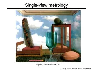
Sample La Flagellazione di Cristo Single View Metrology
Geometry • Overview • Measurements between parallel lines • Measurements on parallel planes • Determining the camera position Single View Metrology
Geometry Overview • Possible to obtain geometric interpretations for key features in a scene • Derive how 3D affine measurements may be extracted from the image • Use results to analyze and/or model the scene Single View Metrology
Assumptions • Assume that images are obtained by perspective projection • Assume that, from the image, a: • vanishing line of a reference plane • vanishing point of another reference direction may be determined from the image Single View Metrology
Geometric Cues • Vanishing Line ℓ • Projection of the line at infinity of the reference plane into the image Single View Metrology
Geometric Cues • Vanishing Point(s) v • A point at infinity in the reference direction • Reference direction is NOT parallel to reference plane • Also known as the vertical vanishing point Single View Metrology
Vertical vanishing point (at infinity) Vanishing line Vanishing point Vanishing point Geometric Cues Single View Metrology
Generic Algorithm • Edge detection and straight line fitting to obtain the set of straight edge segments SA • Repeat • Randomly select two segments s1, s2€ SA and intersect them to give point p • The support set Sp is the set of straight edges in SA going through point p • Set the dominant vanishing point as the point p with the largest support Sp • Remove all edges in Sp from SA and repeat step 2 Single View Metrology
Automatic estimation of vanishing points and lines RANSAC algorithm Candidate vanishing point Single View Metrology
Automatic estimation of vanishing points and lines Single View Metrology
Measurements between Parallel Lines • Wish to measure the distance between two parallel planes, in the reference direction • The aim is to compute the height of an object relative to a reference Single View Metrology
Cross Ratio • Point b on plane ∏ correspond to point t on plane ∏’ • Aligned to vanishing point v • Point i is the intersection with the vanishing line Single View Metrology
Cross Ratio • The cross ratio is between the points provides an affine length ratio • The value of the cross ratio determines a ratio of distances between planes in the world • Thus, if we know the length for an object in the scene, we can use it as a reference to calculate the length of other objects Single View Metrology
Estimating Height • The distance || tr – br || is known • Used to estimate the height of the man in the scene Single View Metrology
Measurements on Parallel Planes • If the reference plane is affine calibrated, then from the image measurements the following can be computed: • Ratios of lengths of parallel line segments on the plane • Ratios of areas on the plane Single View Metrology
Parallel Line Segments • Basis points are manually selected and measured in the real world • Using ratios of lengths, the size of the windows are calculated Single View Metrology
Planar Homology • Using the same principals, affine measurements can be made on two separate planes, so long as the planes are parallel to each other • A map in the world between parallel planes induces a map between images of points on the two planes Single View Metrology
Homology Mapping between Parallel Planes • A point X on plane ∏ is mapped into the point X’ on ∏’ by a parallel projection Single View Metrology
Planar Homology • Points in one plane are mapped into the corresponding points in the other plane as follows: X’ = HX where (in homogeneous coordinates): • X is an image point • X’ is its corresponding point • H is the 3 x 3 matrix representing the homography transformation Single View Metrology
Measurements on Parallel Planes • This means that we can compare measurements made on two separate planes by mapping between the planes in the reference direction via the homology Single View Metrology
Parallel Line Segments lying on two Parallel Planes Single View Metrology
Camera Position • Using the techniques we developed in the previous sections, we can: • Determine the distance of the camera from the scene • Determine the height of the camera relative to the reference plane Single View Metrology
Camera Distance from Scene • In Measurements between Parallel Lines, distances between planes are computed as a ratio relative to the camera’s distance from the reference plane • Thus we can compute the camera’s distance from a particular frame knowing a single reference distance Single View Metrology
Camera Position Relative to Reference Plane • The location of the camera relative to the reference plane is the back-projection of the vanishing point onto the reference plane Single View Metrology
Algebraic Representation • Overview • Measurements between parallel lines • Measurements on parallel planes • Determining the camera position Single View Metrology
Overview • Algebraic approach offers many advantages (over direct geometry): • Avoid potential problems with ordering for the cross ratio • Minimal and over-constrained configurations can be dealt with uniformly • Unifies the different types of measurements • Are able to develop an uncertainty analysis Single View Metrology
Coordinate Systems • Define an affine coordinate system XYZ in space • Origin lies on reference plane • X, Y axes span the reference plane • Z axis is the reference direction • Define image coordinate system xy • y in the vertical direction • x in the horizontal direction Single View Metrology
Coordinate Systems Single View Metrology
Projection Matrix • If X’ is a point in world space, it is projected to an image point x’ in image space via a 3 x 4 projection matrix P • x’ = PX’ = [ p1 p2 p3 p4 ]X’ where x’ and X’ are homogeneous vectors: x’ = (x, y ,w) and X’ = (X, Y, Z, W) Single View Metrology
Vanishing Points • Denote the vanishing points for the X, Y and Z directions as vX, vY, and v • By inspection, the first 3 columns of matrix P are the vanishing points: • p1 = vX • p2 = vY • p3 = v • Origin of the world coordinate system is p4 Single View Metrology
Vanishing Line • Furthermore, vX and vY are on the vanishing line l • Choosing these points fixes the X and Y affine coordinate axes • Denote them as l1 , l2 where li · l = 0 • Note: • Columns 1, 2 and 4 make up the reference plane to image homography matrix H T T T Single View Metrology
Projection Matrix Redux • o = p4 = l/||l|| = l^ • o is the Origin of the coordinate system • Thus, the parametrization of P is: P = [ l1l2αv l^ ] T T αis the affine scale factor Single View Metrology
Measurements between Parallel Lines • The aim is to compute the height of an object relative to a reference • Height is measured in the Z direction Single View Metrology
Measurements between Parallel Lines • Base point B on the reference plane • Top point T in the scene b = n(Xp1 + Yp2 + p4) t = m(Xp1 + Yp2 + Zp3 + p4) n and m are unknown scale factors Single View Metrology
Affine Scale Factor • If α is known, then we can obtain Z • If Z is known, we can compute α, removing affine ambiguity Single View Metrology
Representation Single View Metrology
Measurements on Parallel Planes • Projection matrix P from the world to the image is defined with respect to a coordinate frame on the reference plane • The translation from the reference plane to another plane along the reference direction can be parametrized into a new projection matrix P’ Single View Metrology
Plane to Image Homographies P = [ l1l2αv l^ ] P’ = [ l1l2αv αZv + l^ ] where Z is the distance between the planes T T T T Single View Metrology
Plane to Image Homographies • Homographies can be extracted: H = [ p1 p2αZv + l^] H’ = [ p1 p2l^] • Then H” = H’H-1 maps points from the reference plane to the second plane, and so defines the homology Single View Metrology
Generic Algorithm • Given an image of a planar surface estimate the image-to-world homography matrix H • Repeat • Select two points x1 and x2 on the image plane • Back-project each image point into the world plane using H to obtain the two world points X1 and X2 • Compute the Euclidean distance dist(X1, X2) • dist(A, B) = || A – B || Single View Metrology
Camera Position • Camera position C = (Xc, Yc, Zc, Wc) • PC = 0 • Implies: • Using Cramer’s Rule: Single View Metrology
Camera In Scene Single View Metrology
Uncertainty Analysis • Errors arise from the finite accuracy of the feature detection and extraction • ie- edge detection, point specifications • Uncertainty analysis attempts to quantify this error Single View Metrology
Uncertainty Analysis • Uncertainty in • Projection matrix P • Top point t • Base point b • Location of vanishing line l • Affine scale factor α • As the number of reference distances increases, so the uncertainty decreases Single View Metrology