Download
1 / 29
530 likes | 920 Views
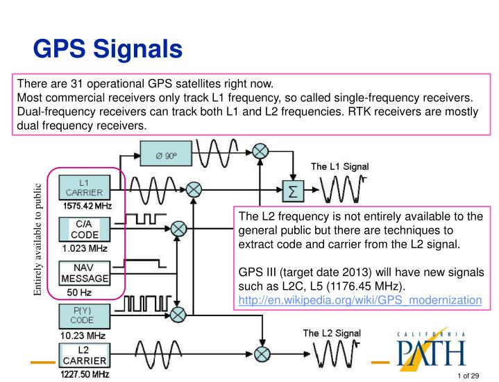
GPS Signals. There are 31 operational GPS satellites right now. Most commercial receivers only track L1 frequency, so called single-frequency receivers. Dual-frequency receivers can track both L1 and L2 frequencies. RTK receivers are mostly dual frequency receivers.

E N D
GPS Signals There are 31 operational GPS satellites right now. Most commercial receivers only track L1 frequency, so called single-frequency receivers. Dual-frequency receivers can track both L1 and L2 frequencies. RTK receivers are mostly dual frequency receivers. The L2 frequency is not entirely available to the general public but there are techniques to extract code and carrier from the L2 signal. GPS III (target date 2013) will have new signals such as L2C, L5 (1176.45 MHz). http://en.wikipedia.org/wiki/GPS_modernization Entirely available to public
Distance Measurement (1/2) Approximated or ignored. Satellite sends models for this. Unknown 1 Approximated. In DGPS, the base station sends this info. Approximated or ignored. Approximated or ignored.
Distance Measurement (2/2) P sr= c * dt c [speed of light] dt [time of flight of C/A signal] AGPS sends this info. GPS can also decode from sky, takes >30 sec and need high SNR. Unknown 4 Unknown 2 Unknown 3 Thus, there are 4 unknowns, need measurements from 4 satellites to solve.
Carrier-Phase (1/2) • Finding travel time using raw carrier signal is more accurate than using C/A code. • L1 carrier frequency = 1.575 GHz, λ = 19 cm • C/A frequency= 1.024 MHz λ = 293 m • This method is counting the exact number of carrier cycles between the satellite and the receiver. • The problem is phase ambiguity. The trick with "carrier-phase GPS" is to use code-phase techniques to get close. If the code measurement can be made accurate to say, a meter, then we only have a few wavelengths of carrier to consider as we try to determine which cycle really marks the edge of our timing pulse [1]. [1] http://www.trimble.com/gps/dgps-advanced4.shtml
Carrier-Phase (2/2) - + The main challenge
Jay Farrell, Tony Givargis, and Matthew Barth, “Real-Time Differential Carrier Phase GPS-Aided INS”, IEEE Trans. On Control Systems Technology, Vol. 8, No. 4, 2000. Shahram Rezaei California PATH, UC Berkeley April 30, 2009
Abstract • Real-time carrier phase differential GPS • To enable advanced vehicle control and safety systems (AVCSS) for intelligent transportation Systems • The implementation achieves 100-Hz vehicle state estimates • Position accuracies at the centimeter level • The amusement park ride experiment demonstrated that the position accuracy was better than 6.0 cm, but beyond this level, the navigation system error could not be discriminated from the mechanical system trajectory error. • For this experiment, the instrument platform was attached to one of the cars on an amusement park ride. The ride has three intended types of rotational motion. For the experiments described below, two degrees of freedom were fixed so that, nominally, the navigation system follows a circular path inclined to the surface of the earth at about 15 .
How they solve phase ambiguity?(1/3) The two basic outputs of a GPS receiver are pseudo-range and carrier phase:
How they solve phase ambiguity?(2/3) • The interest in the carrier signal stems from the fact that the non-common (between receiver and the base station) mode errors and are much smaller than the respective errors on the code range observables. • The common-mode errors are essentially the same as those on the code range observable, except that the ionospheric error enters (3) and (4) with opposite signs. • Therefore, to take advantage of the small non-common mode phase errors, the common mode phase errors must be removed. • This is accomplished through differential operation.
Y. Feng, C. Rizos,“Network-based Geometry-Free Three Carrier Ambiguity Resolution and Phase Bias Calibration”, GPS Solutions, 2009. Shahram Rezaei California PATH, UC Berkeley April15, 2009
The Paper: Motivation The key limitation of existing dual frequency ambiguity resolution (AR) are the constrained service distances between reference stations and user receivers due to the impact of distance-dependent biases such as orbit error, and Ionospheric and Tropospheric signal delay. This has restricted the reference-user receiver distance to about 20km or less in the single-base RTK case (Rizos & Han, 2003). In current network-RTK implementations, the inter-station distance is typically 70km to 90km. This means for a large area like Bay Area (7000 square miles) would reach a few hundreds, representing millions of dollars in installation costs, and significant manual operations costs. Use of multiple-frequency GNSS signals (GPS III) could possibly redefine future RTK services on both a regional and global basis. The reference stations equipped with triple-frequency GNSS receivers may be spaced up to a few hundred kilometers apart, to provide differential and RTK services in regional and rural areas
Three Carrier Ambiguity Resolution (TCAR) This paper describes a geometry-free model for TCAR and phase bias estimation with DD (Double Difference) and ZD (Zero Difference) code and phase measurements for network-based data processing. Double Difference observation is formed by subtracting two single difference observations for two satellites at the same time. Geometry of 4 DD and 9 ZD measurements Single Difference Observation
Basic Equations To begin with, we define the observation equations for the virtual phase and code measurements in meters: scale factor Cycle ambiguity initial phase of the receiver oscillator in cycles, receiver dependant ionospheric propagation delay with respect to L1 phase wavelength Receiver clock error in sec Speed of light Satellite clock error in sec initial phase of the satellite oscillator in cycles, satellite dependant tropospheric propagation delay in m noise geometric distance between satellite S and receiver antenna R orbit error, satellite dependant A linear combination of three fundamental signals f1, f2, and f3: Carrier frequencies for L1, L2 and L5 signals. (i,j, k) and (l, m, n) are integer coefficients
Basic Equations The double-differenced (DD) phase and code measurements are:
General formation of geometry-free TCAR models (1/4) The geometry-free observational model for a virtual integer parameter is generally expressed as: In this Eq., (l, m, n) and (i, j, k) generally are different sets of integer values, representing various possible combinations between them. Code and phase signals that are minimally affected by the joint ionospheric term, code and phase noises, with respect to their virtual wavelengths, should be considered the better choices for AR purposes.
General formation of geometry-free TCAR models (2/4) Three traditional choices are the WLs which the ionospheric term cancels, and the effects of the code noise term are nearly at a minimum. However, it is possible to find more useful signals for AR purpose under different ionospheric and noise conditions.
General formation of geometry-free TCAR models (3/4) In general, the first ambiguity is determined as: After the first two EWL/WL signals are resolved, it is time to estimate the ionospheric bias. The formula with the two WLs is given as follows:
General formation of geometry-free TCAR models (4/4) The third virtual signal can be chosen from a new category, of which any combination is linearly independent of the previous two EWL/WL virtual signals. This paper chooses the L1 phase measurement as the third virtual signal, whose ambiguity is determined by averaging over K epochs.
Geometry-free TCAR models for LAMBDA integer estimation (1/4) More generally, one can formulate the geometry-free TCAR problem as a linear observation equation:
Geometry-free TCAR models for LAMBDA integer estimation (2/4) In the dual-frequency case: For a network numbering n stations with m satellites in common view, there will be M sets of DD measurements, where M=(n-1)(m-1).
Geometry-free TCAR models for LAMBDA integer estimation (3/4)
Geometry-free TCAR models for LAMBDA integer estimation (4/4)
Three carrier phase-bias estimation for ZD phase measurements (1/5) Code and phase signals with minimal effects due to ionospheric delays and code and phase noises, should be considered the best choice for the estimation of the phase bias term. However, the key problem is the ionospheric delay in the slant path ZD measurements, which is of the order of metres to tens of metres. In some combinations, the ionospheric term cancels; however, those are not useful for positioning without removing the ionosphere bias. Therefore one chooses the ionosphere-free combination.
Three carrier phase-bias estimation for ZD phase measurements (2/5) In dual frequency case:
Three carrier phase-bias estimation for ZD phase measurements (3/5) The traditional approach is to perform simple averaging for the phase biases in above equations separately. A more rigorous approach is the least squares estimation procedure described below: At epoch k, the generalised linear equations for all n stations and m satellites are expressed as: Finally, we can find the least-square estimate over K epochs:
Three carrier phase-bias estimation for ZD phase measurements (4/5) The next procedure is a network-adjustment approach which considers the DD integer constraints. If the DD integer ambiguities can be resolved, the known DD integers can be used to improve the estimates of the ZD phase biases, taking advantage of multiple stations and high quality measurements from some stations in the network. In general, given the 3nm-by-1 ZD phase bias vector YN which represents the virtual observational vector from the estimated Nhat with the noise vector , the following linear equation and statistical conditions are obtained: The least-squares solution is: where D is the double-difference operator matrix.
Three carrier phase-bias estimation for ZD phase measurements (5/5) Illustration of the convergence of various magnitudes of the initial ZD phase bias errors (single epoch) versus the filtering time (epochs) under zero mean and white noise conditions.