Download

1 / 25
250 likes | 382 Views
An idealized semi-empirical framework for modeling the MJO. Adam Sobel and Eric Maloney. NE Tropical Workshop, May 17 2011. A set of postulates about MJO dynamics. Not a Kelvin wave (though may have something to do with Kelvin waves) A moisture mode – meaning moisture field is critical

E N D
An idealized semi-empirical framework for modeling the MJO Adam Sobel and Eric Maloney NE Tropical Workshop, May 17 2011
A set of postulates about MJO dynamics • Not a Kelvin wave (though may have something to do with Kelvin waves) • A moisture mode – meaning moisture field is critical • Destabilized by feedbacks involving surface turbulent fluxes and radiative fluxes • Horizontal moisture advection important to the dynamics (wind speeds ≥ propagation speed)
A set of postulates about MJO dynamics • Not a Kelvin wave (though may have something to do with Kelvin waves) • A moisture mode – meaning moisture field is critical • Destabilized by feedbacks involving surface turbulent fluxes and radiative fluxes • Horizontal moisture advection important to the dynamics (wind speeds ≥ propagation speed) These postulates are supported by a lot of evidence from observations and comprehensive numerical models. E.g…
Aquaplanet GCM simulation with warm pool Control No-WISHE • WISHE appears to destabilize the MJO in the model. 30-90 day, zonal wavenumber 1-3 variance decreases dramatically without WISHE active • Horizontal moisture advection plays large role in propagation (not shown)
A convectively coupled Kelvin wave can only be destabilized by WISHE if mean surface winds are easterly (Emanuel 1987; Neelin et al. 1987) If the MJO is not a Kelvin wave, then no theory forbids WISHE acting in mean westerlies (as exist in warm pool) But in mean westerlies, WISHE will tend to induce westward propagation, because strongest winds to west of convection. How might an eastward-propagating moisture mode, destabilized by WISHE in mean westerlies, work?
Our approach, conceptually: • Start from a single-column model under the weak • temperature gradient approximation. • Quasi-equilibrium convective physics, simple • cloud-radiative feedbacks. (This allows a representation of • convective self-aggregation as in CRMs) Bretherton et al. 2005
Our approach, conceptually: • Start from a single-column model under the weak • temperature gradient approximation. • Quasi-equilibrium convective physics, simple • cloud-radiative feedbacks. (This allows a representation of • convective self-aggregation as in CRMs). • Add a horizontal dimension (longitude). Assume wind is • related diagnostically to heating by simple Gill-type dynamics • (or something close to that):
Gill (1980) wind and geopotential for localized heating (at 0,0) linear, damped, steady dynamics on equatorial beta plane Zonal wind response to delta function heating Zonal wind response (red) to sinusoidal heating (blue)
Our approach, conceptually: • Start from a single-column model under the weak • temperature gradient approximation. Only prognostic variable • is column-integrated water vapor. • Quasi-equilibrium convective physics, simple • cloud-radiative feedbacks. (This allows a representation of • convective self-aggregation as in CRMs). Gross moist stability • is constant (or parameterized…) • Add a horizontal dimension (longitude). Assume wind is • related diagnostically and instantaneously to heating, e.g. • by simple Gill-type dynamics • 4. Allow wind to advect moisture, and influence surface fluxes. in results shown here E depends on u only
Compute u from a projection operator: Using Gill dynamics (almost): L depends on equivalent depth and damping rate. We cheat sometimes and shift G relative to forcing by a small amount, δ - ascribed to missing processes in Gill model (CMT, nonlinearity…)
Model is 1D, represents a longitude line at a single latitude, where the MJO is active. But we do not assume that the divergence = u/x. (there is implicit meridional structure, v/y ≠ 0) Relatedly, the mean state is not assumed to be in radiative-convective equilibrium. Rather it is in weak temperature gradient balance. Zonal mean precip is part of the solution. Implicitly there is a Hadley cell.
All linear modes are unstable due to WISHE, but westward- propagating Most unstable wavelength is ~decay length scale for stationary response to heating L (c/ε, where ε is damping rate; here 1500 km)
Nonlinear model configuration details • 1D domain 40,000 km long, periodic boundaries • Background state is uniform zonal flow – eastward at 5 m/s; perturbation flow is added to it for advection and surface fluxes. • In simulations shown below normalized gross moist stability = 0.1; cloud radiative feedback = 0.1; saturation column water vapor =70 mm; these factors largely control stability;
Nonlinear behavior is or is not qualitatively similar to linear, depending on wind response shift δ Saturation fraction vs. longitude and time, for different values of δ
With a small adjustment to the wind response to heating (westerlies a little further east) we get very nonlinear behavior Perturbation zonal wind; total is that plus mean 5m/s. Relative strength of easterlies and westerlies is tunable.
This semi-empirical model is not a satisfactory theory for the MJO, • yet. It is a framework within which the consequences of several • ideas can be explored. • Key parameters: • The gross moist stability • Cloud-radiative feedback • Mean state – zonal wind and mean rainfall/divergence • The quasi-steady wind response to a delta function heating (G) – • very sensitive to small longitudinal shifts! • These can all - in principle - be derived from/tuned to diagnostics of • global models. • We see that very nonlinear behavior can emerge (and can go eastward). • Working on: mixed layer ocean coupling, variable gross moist stability…
Vertically integrated equations for moisture and dry static energy, under WTG approximation ± is upper tropospheric divergence. Add to get moist static energy equation Substitute to get where is the “normalized gross moist stability”
Our physics is semi-empirical: The functional forms chosen are key components of the model - and hide much implicit vertical structure. We do explicitly parameterize at this point R = max(R0-rP, 0) with R0, r constants. Substituting into the MSE equation and expanding the total derivative, (for sake of argument assuming rP<R0) “effective” NGMS (including cloud-radiative feedback) u is the zonal wind at a a nominal steering level for W, presumably lower-tropospheric.
We parameterize precipitation on saturation fraction by an exponential (Bretherton et al. 2004): (with e.g., ad=15.6, rd=0.603), and R is the saturation fraction, R=W/W*. Here W*, the saturation column water vapor, is assumed constant as per WTG. We represent the normalized GMS either as a constant or as a specified function of W. NGMS is very sensitive to vertical structure and so the most important (implicit) assumptions about vertical structure are buried here.
Rather than use a bulk formula for E, we go directly to the simulations of Maloney et al. A scatter plot of E vs. U850 in the model warm pool yields the parameterization E = 100 + 7.5u With E in W/m2 and u in m/s. Note there is no dependence on W or SST. In practice it assures that simple model does not have very different wind-evaporation feedback than the GCM.
Variance of rainfall on intraseasonal timescales shows structure on both global and regional scales Intraseasonal rain variance Northern Summer Southern Summer Sobel, Maloney, Bellon, and Frierson 2008: Nature Geosci.,1, 653-657.
Climatological patterns resemble variance, except that the mean doesn’t have localized minima over land Intraseasonal OLR variance (may-oct) Climatological mean OLR (may-oct)
Climatological patterns resemble variance, except that the mean doesn’t have localized minima over land Intraseasonal OLR variance, nov-apr Climatological mean OLR, nov-apr
Emanuel (87) and Neelin et al. (87) proposed that the MJO is a Kelvin wave driven by wind-induced surface fluxes (“WISHE”) θ=θ1+Δθ θ=θ1 cool warm Enhanced sfc flux Mean flow Perturbation flow Wave propagation
Instead we propose a moisture mode driven by surface flux feedbacks Warm θ=θ1+Δθ Mean + perturbation flow θ=θ1 Enhanced sfc flux humid dry Mean flow Perturbation flow (partly rotational) Disturbance propagation (via horizontal advection…)