Download

1 / 42
420 likes | 421 Views
AME 436 Energy and Propulsion. Lecture 9 Unsteady-flow (reciprocating) engines 4: Non-ideal cycle analysis. Outline. AirCyclesForRecips.xls spreadsheet - how it works and how to use it Some non-ideal effects Irreversible compression/expansion Heat transfer to gas during cycle

E N D
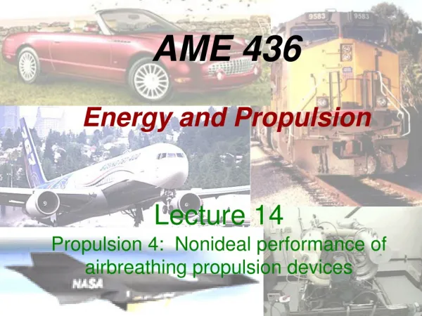
AME 436Energy and Propulsion Lecture 9 Unsteady-flow (reciprocating) engines 4: Non-ideal cycle analysis
Outline • AirCyclesForRecips.xls spreadsheet - how it works and how to use it • Some non-ideal effects • Irreversible compression/expansion • Heat transfer to gas during cycle • Finite burn time / spark advance • Exhaust residual • Friction • Factors that limit maximum RPM • Performance plots - Power & Torque vs. RPM AME 436 - Spring 2019 - Lecture 9 - Non-ideal cycle analysis
AirCycles4Recips.xls • Thermodynamic model isexact, but heat loss, burn rate, etc. models are qualitative • Constant not realistic (changes from ≈ 1.4 to 1.25 during the cycle) but only affects results quantitatively (not qualitatively) (1 of 2 most significant weaknesses of AirCycles4Recips.xls) • Heat transfer model • T ~ h(Twall -Tgas), where dimensionless heat transfer coefficient (h) & cylinder wall temperature (Twall) are specified constants - physically reasonable • h is a "Sherwood number" = h/CPLN, where h is the dimensional heat transfer coefficient (W/m2K) and L is a characteristic dimension (e.g. cylinder diameter) (LN is a characteristic velocity; if L = stroke then LN = mean piston speed) • Increments each cell not each time step • Doesn't include effects of varying area, varying turbulence, varying time scale through piston motion, etc. on h AME 436 - Spring 2019 - Lecture 9 - Non-ideal cycle analysis
AirCycles4Recips.xls • Work transfer from step i to step i+1 W = Q - dU (1st Law of Thermo, conservation of energy) Q = Cvh(Twall -Ti) + (f)QR/Cv dU = Ui+1 - Ui = Cv(Ti+1 - Ti) (constant CV) f = increment of fuel burned in current step • Friction loss is a specified FMEP • Use latest version from AME 436 website - some plots embedded in lecture notes were built with earlier versions • Model considers only 1 gas in cylinder - improved model should consider 2 separate gases, burned & unburned, with combustion increasing amount of burned gas(2nd significant weakness of AirCycles4Recips.xls) AME 436 - Spring 2019 - Lecture 9 - Non-ideal cycle analysis
AirCycles4Recips.xls - intake process • Intake process spread across 25 Excel cells (i = 1, 2, … 25) ; 1/25 of total cylinder volume increase in each successive cell • Pressure Pintake & specific volume vintake assumed constant • In first row of intake process • If "Exhaust Residual" = FALSE then T = Tintake • If "Exhaust Residual" = TRUE then T = final exhaust temperature after expansion, blowdown, and intake start • If "Exhaust residual" = TRUE, iteration required since the exhaust temperature is not known until the end of the cycle; use SOLVE button to update solution after changing any input parameter (otherwise SOLVE button does nothing) • After first row Tintake = T of the fresh gas but it mixes with gas already in cylinder that has different T due to heat loss /gain; mixed gas T conserves internal energy of fresh + existing charge: (mi+1)CvTi+1 = miCvTi + mCvTintake where m = mi+1 - mi = (Vi+1-Vi)/vintake = (Vi+1-Vi)/(RTintake/ Pintake) AME 436 - Spring 2019 - Lecture 9 - Non-ideal cycle analysis
AirCycles4Recips.xls - compression • Compression spread across 25 cells; 1/25 of total cylinder volume decrease in each successive cell • Done in two steps: (1) Wall heat transfer at constant volume (2) Adiabatic compression according to the usual PV relations; may be irreversible according to (see lecture 7, pages 17-18) comp = 1 reversible adiabatic process • Compression ends at volume Vc + Vd*BurnStart, where BurnStart is a specified number (0 ≤ BurnStart < 1) • BurnStart must be ≥ 0, i.e. combustion must start at or before minimum volume (a limitation of the spreadsheet, not a fundamental limitation of cycles) • If BurnStart > 0, some compression occurs during heat addition step (next…) AME 436 - Spring 2019 - Lecture 9 - Non-ideal cycle analysis
AirCycles4Recips.xls - combustion • Same two-step process of heat transfer at constant V + adiabatic compression, but now both heat transfer to/from wall AND heat input due to combustion f = fraction of fuel burned during step • By default (Burn Rate Profile = 0) f = f/25, but can use Burn Rate Profile > 0 or < 0 to have more burning near end (realistic) or beginning (unrealistic) of combustion process AME 436 - Spring 2019 - Lecture 9 - Non-ideal cycle analysis
AirCycles4Recips.xls - combustion • If BurnStart > 0 then compression continues (with combustion) until minimum cylinder volume (= Vc) • Heat addition ends at volume Vc + Vd*BurnEnd, where BurnEnd is specified (0 ≤ BurnEnd < 1) • Note two stages of heat addition corresponding to volumes: (1) Vc + Vd*BurnStartVc (2) VcVc + Vd*BurnEnd • If BurnEnd > 0, expansion occurs in conjunction with heat addition • As with BurnStart, BurnEnd must be ≥ 0, i.e. combustion must end at or after minimum cylinder volume • If "Const V comb?" = FALSE, constant pressure combustion is calculated (Diesel cycle); BurnStart, BurnEnd, BurnRateProfile have no effect and (Same as before but with CP instead of Cv, and volume (v) increasing rather than constant) AME 436 - Spring 2019 - Lecture 9 - Non-ideal cycle analysis
Expansion process • Expansion spread across 25 cells; 1/25 of total cylinder volume increase in each successive cell • Done in two steps (1) Wall heat transfer at constant V as usual (2) Adiabatic expansion according to the usual PV relations but may be irreversible according to • Followed by expansion to P = Pexhaust = Pambient if "Complete Expansion" = TRUE; same heat transfer & expansion laws apply AME 436 - Spring 2019 - Lecture 9 - Non-ideal cycle analysis
Blowdown, exhaust processes • "Blowdown" or "blowup" is assumed isentropic, infinitely fast so no heat transfer; not applicable if complete expansion (already at ambient pressure) • Exhaust process • Spread across 25 cells; 1/25 of total cylinder volume decrease in each successive cell • Pexhaust assumed constant • Heat transfer may occur as usual (exhaust heat transfer only affects cycle performance if "Exhaust Residual" = TRUE) AME 436 - Spring 2019 - Lecture 9 - Non-ideal cycle analysis
Irreversible (but adiabatic) comp / exp • If piston expands infinitely fast, no work done (piston outruns gas molecules), no work done; if piston compresses too fast, builds up shocks • Not important except at very high RPM (choking at valves), important for propulsion at M2 close to or larger than 1 • P-V diagram - for same V, more P during compression Red solid: comp = exp = 1 Blue dashed: comp = exp = 0.5 r = 3, = 1.3, f = 0.01, QR = 4.5 x 10⁷ J/kg, Tin = 300K, Pin = 1 atm, Pexh = 1 atm. ExhRes = FALSE, Const-v comb = TRUE, BurnStart = BurnEnd = BurnRateProfile = 0, ComplExp = FALSE, h = 0, comp = exp = 0.5 or 1 AME 436 - Spring 2019 - Lecture 9 - Non-ideal cycle analysis
Irreversible (but adiabatic) comp / exp • Larger change in T-s diagram - for same V, more T ( more work) during compression, less T ( less work) during expansion since s > 0 with irreversible compression/expansion (see lecture 6) • Significant effect on th = 0.281 (comp = exp = 1) vs. 0.211 (comp = exp = 0.9) for case shown (note I used comp = exp = 0.5 for P-V diagram) Red solid: comp = exp = 1 Blue dashed: comp = exp = 0.9 r = 3, = 1.3, f = 0.01, QR = 4.5 x 10⁷ J/kg, Tin = 300K, Pin = 1 atm, Pexh = 1 atm. ExhRes = FALSE, Const-v comb = TRUE, BurnStart = BurnEnd = BurnRateProfile = 0, ComplExp = FALSE, h = 0, comp = exp = 0.9 or 1 AME 436 - Spring 2019 - Lecture 9 - Non-ideal cycle analysis
Irreversible (but adiabatic) comp / exp • Moderate irreversibility in compression doesn't hurt much (just a little more compression work) but irreversibility in expansion directly deducts from net work; though severe compression irreversibility hurts more • (Obviously) combined compression & expansion irreversibility is worst r = 8, = 1.3, f = 0.068, QR = 4.5 x 10⁷ J/kg, Tin = 300K, Pin = 1 atm, Pexh = 1 atm. ExhRes = FALSE, Const-v comb = TRUE, BurnStart = BurnEnd = BurnRateProfile = 0, ComplExp = FALSE, h = 0, comp = variable, exp = variable AME 436 - Spring 2019 - Lecture 9 - Non-ideal cycle analysis
Heat transfer during cycle • More P during compression - T higher due to heat transfer in - more work required to compress higher-T gas for same V3/V2 w = mCv(T2 - T3) = mCvT2(1 - T3/T2) = mCvT2 [ 1 - (V2/V3)-1 ] • Less P during combustion - heat loss decreases T thus P for fixed V • P falls faster during expansion - heat loss - less work for same V5/V4 Red solid: h = 0 Blue dashed: h = 0.015, Twall = 400K r = 3, = 1.3, f = 0.01, QR = 4.5 x 10⁷ J/kg, Tin = 300K, Pin = 1 atm, Pexh = 1 atm ExhRes = FALSE, Const-v comb = TRUE, BurnStart = BurnEnd = BurnRateProfile = 0 ComplExp = FALSE, h = 0 or 0.015, Twall = 400K, comp = exp = 1 AME 436 - Spring 2019 - Lecture 9 - Non-ideal cycle analysis
Heat transfer during cycle • Const. P heat addition during intake, so higher T & s than adiabatic cycle • Heat addition during 1st part of compression (ds > 0), heat loss (ds < 0) during 2nd part of compression & rest of cycle • Still const. V combust., so same const.-v curve but less T due to heat loss • Significant effect on th - 0.281 (h = 0) vs. 0.177 (h = 0.015) for case shown Red solid: h = 0 Blue dashed: h = 0.015, Twall = 400K Wall T r = 3, = 1.3, f = 0.01, QR = 4.5 x 10⁷ J/kg, Tin = 300K, Pin = 1 atm, Pexh = 1 atm ExhRes = FALSE, Const-v comb = TRUE, BurnStart = BurnEnd = BurnRateProfile = 0 ComplExp = FALSE, h = 0 or 0.015, Twall = 400K, comp = exp = 1 AME 436 - Spring 2019 - Lecture 9 - Non-ideal cycle analysis
Heat transfer during cycle • Obviously, increasing heat loss coefficient h decreases th • Wall T has almost no effect for fixed h - extra heat transfer in during compression (thus more work in) at high T is balanced by more heat transfer during expansion (thus more work out) r = 8, = 1.3, f = 0.068, QR = 4.5 x 10⁷ J/kg, Tin = 300K, Pin = 1 atm, Pexh = 1 atm ExhRes = FALSE, Const-v comb = TRUE, BurnStart = BurnEnd = BurnRateProfile = 0 ComplExp = FALSE, h = variable, Twall = variable, comp = exp = 1 AME 436 - Spring 2019 - Lecture 9 - Non-ideal cycle analysis
Heat transfer scaling estimate • Heat transfer (Q) to a wall at temperature Tw from a slab of gas of thickness x, area A & temperature Tg (initially at Tg,ad) Q = kA(T/x) = kA((Tg-Tw)/x) • Rate of decrease of enthalpy of said slab Q = mCP(T/t) = VCP((Tg,ad-Tg)/t) = AxCP(Tg,ad-Tg)/t • Equate: (k/CP)(Tg-Tw)/(Tg,ad-Tg) = (Tg-Tw)/(Tg,ad-Tg) = (x)2/t or "Importance of heat losses" ~ (Tg,ad-Tg)/(Tg-Tw) ~ t/(x)2 • For turbulent flow, ~ u'LI • In an engine, u' ~ upiston ~ SN (S = stroke ~ x, N = RPM), LI ~ S ~ x,t ~ 1/N • Combining these, (Tg-Tw)/(Tg-T∞) ~ constant(independent of engine size (x) and rotation rate (N)) • If not turbulent (very low Re, Ii.e. very low speed or very small engine), ≈ constant (not a function of u’ and LI) then "Importance of heat losses" ~ /NS2 AME 436 - Spring 2019 - Lecture 9 - Non-ideal cycle analysis
Heat transfer - mini-catechism • Why do we have heat loss in engines? Because the cylinder wall is “cold” - typically just a little higher than the cooling water temperature, ≈ 120˚C (boiling point at 2 atm). This is much colder than the gases during combustion (2400K) and during expansion (down to 1200K). • Why do we need to cool the cylinder? To keep the lubricating oil from getting too hot and breaking down. Also, with too large a temperature increase, thermal expansion will change the fit between the piston and cylinder and make it too tight or too loose. • How significant is the loss? See Heywood Fig. 12-4: At low vehicle speed (meaning: low engine RPM, low Pintake) 50% of fuel energy is dissipated as cooling system losses; at higher speed, 30%; Heywood (p. 851) states that a 10% decrease in heat loss would mean about 3% increase in BMEP • Could we reduce the loss by using a ceramic (or whatever material) engine that could withstand high temperatures without oil lubrication? The analysis 2 pages back shows that raising Twalldoesn’t increase efficiency; what is needed is a more nearly adiabatic engine (lower h). This is borne out by many experiments, peaking in the 1980's, using so-called "adiabatic" or “low heat rejection” engines made of ceramics. This raised Twall but caused more heat transfer during compression, thereby increasing compression work, so the efficiency didn’t improve. AME 436 - Spring 2019 - Lecture 9 - Non-ideal cycle analysis
Heat transfer - mini-catechism • How can we decrease h? Heat transfer in engines is controlled by turbulence, so you need to decrease turbulence • How can you do that? Engines are designed for high turbulence, so you could reverse-engineer the engine for lower turbulence (e.g. by avoiding swirl in the intake ports, using "anti-squish" (see lecture 4), etc.) • Why don't we do that now? Because we need high turbulence (high u') to get fast burning • Is there any way to burn fast without turbulence? I'm working on that; one possibility is transient plasma ignition, which produces multiple streamers of electrons, thus multiple ignition sites, for one set of electrodes Cylinder pressure (lb/in2) AME 436 - Spring 2019 - Lecture 9 - Non-ideal cycle analysis
Slow burn • For ignition before the minimum volume (Before Top Dead Center, BTDC), P increases faster (since both compression AND burning), but same minimum volume must be reached • Burning After Top Dead Center (ATDC) leads to much lower peak P (some burning during expansion) but somewhat higher P during expansion Red solid: BurnStart = BurnEnd = 0 Blue dashed: BurnStart = 0.1, BurnEnd = 0.1 r = 3, = 1.3, f = 0.01, QR = 4.5 x 10⁷ J/kg, Tin = 300K, Pin = 1 atm, Pexh = 1 atm, BurnRateProfile = 1, ExhRes = FALSE, Const-v comb = TRUE, ComplExp = FALSE, h = 0, Twall = 400K, comp = exp = 1 AME 436 - Spring 2019 - Lecture 9 - Non-ideal cycle analysis
Slow burn • Burn starts earlier in compression process, has to go to same v, result is higher s to get same heat addition (= ∫Tds) • Difference in work: 2 triangular slivers vs. rectangle • Burning BTDC or ATDC ALWAYS leads to lower efficiency since ALWAYS lower TH for same TL, thus ALWAYS lower efficiency Carnot "strips" • Moderate effect on th - 0.281 (Instant burn) vs. 0.242 (slow burn) for case shown Red solid: BurnStart = BurnEnd = 0 Blue dashed: BurnStart = 0.1, BurnEnd = 0.1 r = 3, = 1.3, f = 0.01, QR = 4.5 x 10⁷ J/kg, Tin = 300K, Pin = 1 atm, Pexh = 1 atm, BurnRateProfile = 1, ExhRes = FALSE, Const-v comb = TRUE, ComplExp = FALSE, h = 0, Twall = 400K, comp = exp = 1 AME 436 - Spring 2019 - Lecture 9 - Non-ideal cycle analysis
Slow burn – impact on ideal cycle • How to minimize impact of slow burn? Ignite the mixture BTDC; while this means some mixture is burned too early, and some burns ATDC, th better than if you wait until TDC to start burning Burn Duration BurnStart + BurnEnd r = 8, = 1.3, f = 0.068, QR = 4.5 x 10⁷ J/kg, Tin = 300K, Pin = 1 atm, Pexh = 1 atm ExhRes = FALSE, Const-v comb = TRUE, BurnStart = variable BurnEnd = variable, BurnRateProfile = 0, ComplExp = FALSE, h = 0, comp = exp = 1 AME 436 - Spring 2019 - Lecture 9 - Non-ideal cycle analysis
Slow burn – impact on non-ideal cycle • With ideal cycle (no heat losses, reversible compression & expansion, no exhaust residual) optimal timing ≈ symmetric (BurnStart = BurnEnd), (previous page), but with non-ideal cycle (below), better to start burning slightly later in cycle (less heat losses) Burn Duration BurnStart + BurnEnd r = 8, = 1.3, f = 0.068, QR = 4.5 x 10⁷ J/kg, Tin = 300K, Pin = 1 atm, Pexh = 1 atm BurnRateProfile = 0, ExhRes = TRUE, Const-v comb = TRUE ComplExp = FALSE, h = 0.01, comp = exp = 0.9 AME 436 - Spring 2019 - Lecture 9 - Non-ideal cycle analysis
Slow burn • Rule of thumb: best efficiency when ignition timing chosen so that maximum P occurs ≈ 10˚ ATDC • This spreadsheet: for Burn Duration = 0.15, optimal "timing" is BurnStart = 0.045, BurnEnd = 0.105, more burning ATDC - consistent with real engine • Leaner mixtures: slower burning, need to advance spark more • Spark advance sounds good BUT… • Peak temperature substantially affected - this affects NOx formation greatly - high activation energy (E) and knock (next lecture …) • Minimum peak T when BurnStart < BurnEnd, so that more burning occurs AFTER minimum volume • "Compress then burn" leads to lower T than "burn then compress" - burn ADDS to T, compression MULTIPLIES T • If 1 - 2 is compress, 2 - 3 is burn then T2 = T1r-1; T3 = T2 + fQR/Cv = T1r-1 + fQR/Cv • If 1 - 2 is burn, 2 - 3 is compress then T2 = T1 + fQR/Cv; T3 = T2r-1; = (T1 + fQR/Cv)r-1 • T3(BurnComb)- T3(CompBurn) = (fQR/Cv)(r-1 - 1) > 0 AME 436 - Spring 2019 - Lecture 9 - Non-ideal cycle analysis
Slow burn - effect on peak cycle T • As ignition timing is "advanced" (more burning BTDC, moving to right on plot below), peak cycle T increases substantially • Temperatures are unrealistically high since model assumes constant CP & Cv, no dissociation but the trend will be the same with “real” gases r = 3, = 1.3, f = 0.068, QR = 4.5 x 10⁷ J/kg, Tin = 300K, Pin = 1 atm, Pexh = 1 atm ExhRes = TRUE, Const-v comb = TRUE, BurnStart = variable, BurnEnd = variable BurnRateProfile = 0, ComplExp = FALSE, h = 0.01, comp = exp = 0.9 AME 436 - Spring 2019 - Lecture 9 - Non-ideal cycle analysis
Burn Rate Profile • For more burning at beginning of cycle (BurnRateProfile = -1), more "burn then compress," higher peak pressures • BurnRateProfile > 0 is more realistic since more mass burned late in cycle after pressure (thus density) is higher (SL & ST not affected much by pressure) r = 3, = 1.3, f = 0.01, QR = 4.5 x 10⁷ J/kg, Tin = 300K, Pin = 1 atm, Pexh = 1 atm BurnStart = 0.1, BurnEnd = 0.1, ExhRes = FALSE, Const-v comb = TRUE ComplExp = FALSE, h = 0, Twall = 400K, comp = exp = 1 AME 436 - Spring 2019 - Lecture 9 - Non-ideal cycle analysis
Burn Rate Profile • Very little effect on T-s diagram - same minimum volume reached at different points in cycle • Very little effect on efficiency - 0.244 (BurnRateProfile = 1) vs. 0.241 (BurnRateProfile = -1) for this example r = 3, = 1.3, f = 0.01, QR = 4.5 x 10⁷ J/kg, Tin = 300K, Pin = 1 atm, Pexh = 1 atm BurnStart = 0.2, BurnEnd = 0.2, ExhRes = FALSE, Const-v comb = TRUE ComplExp = FALSE, h = 0, Twall = 400K, comp = exp = 1 AME 436 - Spring 2019 - Lecture 9 - Non-ideal cycle analysis
Exhaust residual • P-V diagram very similar, P2 - P3 is same (but gas going through cycle has higher T) • Peak P decreases since starting at higher T2 P4/P3 = T4/T3 = (T3 + fQR/Cv)/T3 = 1 + fQR/CvT3 = 1 + fQR/CvT2r-1 Red solid: Exh Res = FALSE Blue dashed: Exh Res = TRUE r = 3, = 1.3, f = 0.01, QR = 4.5 x 10⁷ J/kg, Tin = 300K, Pin = 1 atm, Pexh = 1 atm ExhRes = FALSE, Const-v comb = TRUE, BurnStart = 0 or 0.05, BurnEnd = 0 BurnRateProfile = 0, ComplExp = FALSE, h = 0, Twall = 400K, comp = exp = 1 AME 436 - Spring 2019 - Lecture 9 - Non-ideal cycle analysis
Exhaust residual • Higher starting T & s, otherwise ideal cycle • In ideal cycle residual has no effect on th but since exhaust residual has no fuel & lower density (higher v) than fresh gas, power or BMEP is decreased (1.84 atm vs. 2.20 atm for case shown) Red solid: Exh Res = FALSE Blue dashed: Exh Res = TRUE r = 3, = 1.3, f = 0.01, QR = 4.5 x 10⁷ J/kg, Tin = 300K, Pin = 1 atm, Pexh = 1 atm ExhRes = FALSE, Const-v comb = TRUE, BurnStart = 0 or 0.05, BurnEnd = 0 BurnRateProfile = 0, ComplExp = FALSE, h = 0, Twall = 400K, comp = exp = 1 AME 436 - Spring 2019 - Lecture 9 - Non-ideal cycle analysis
Complete cycle, all effects included • Comparison of cycles with "realistic" operating parameters • No throttling in this example • "Spark timing" used provides maximum th for burn duration of 0.15 • Much lower peak P (less than 1/2) for non-ideal cycle • Cycle efficiency: 0.464 vs. 0.293, IMEP 18.9 atm vs. 11.8 atm; BMEP 18.9 atm vs. 10.8 atm (assuming FMEP = 1 atm) Red solid: Ideal cycle Blue dashed: all effects r = 8, = 1.3, f = 0.068, QR = 4.5 x 10⁷ J/kg, Tin = 300K, Pin = 1 atm, Pexh = 1 atm, Const-v comb = TRUE BurnStart = 0 or 0.045, BurnEnd = 0 or 0.105, h = 0 or 0.01, Twall = 400K, comp = exp = 0.9 or 1 AME 436 - Spring 2019 - Lecture 9 - Non-ideal cycle analysis
Complete cycle, all effects included • Cycle starts at higher T & s due to exhaust residual + heating during intake • s increases during compression - irreversible and non-adiabatic • Combustion not at constant V, but eventually hits (almost) same v (slightly lower since not as much mass, thus lower v for same V) • Less T in combustion and lower peak T due to heat loss & combustion not at constant volume Red solid: Ideal cycle Blue dashed: all effects Just coincidence that maximum s is same for both cycles r = 8, = 1.3, f = 0.068, QR = 4.5 x 10⁷ J/kg, Tin = 300K, Pin = 1 atm, Pexh = 1 atm, Const-v comb = TRUE BurnStart = 0 or 0.045, BurnEnd = 0 or 0.105, h = 0 or 0.01, Twall = 400K, comp = exp = 0.9 or 1 AME 436 - Spring 2019 - Lecture 9 - Non-ideal cycle analysis
Friction • Does NOT appear on P-V or T-s diagram • How to measure? • FMEP = IMEP - BMEP: measure IMEP (from P-V diagram) and BMEP (from engine work output to dynamometer); not very accurate since it’s the difference between two nearly equal noisy numbers (e.g. 10 vs. 9 atm) • Motoring test: spin engine with electric motor, measure power needed - but firing engine has different forces/stresses, not so accurate either • Morse test: Remove spark plug wires one at a time, measure BMEP vs. number of firing cylinders, extrapolate to zero firing cylinders, this corresponds to IMEP = 0, BMEP will be < 0, thus BMEP = -FMEP AME 436 - Spring 2019 - Lecture 9 - Non-ideal cycle analysis
Friction • Typical result: FMEP increases roughly as N1/2; since friction power = FMEP*N*Vd /n, friction power ~ N1.5, thus at higher N, a higher % of IMEP is lost to friction (see Heywood Fig. 13-6 - 13-13) • Typical values for automotive-size engines: FMEP ≈ 1 atm at N = 500 RPM, increasing to 2.5 atm at N = 5000 RPM • Not strongly dependent on IMEP (i.e. Pintake) for given N Heywood (1988) AME 436 - Spring 2019 - Lecture 9 - Non-ideal cycle analysis
Factors that limit RPM (thus power) • Mechanical strength of parts (obviously…) • Choking at valves - as N increases, mass flow ( ) needed to fill cylinder increases, but for fixed intake valve area A*, upstream pressure Pt and temperature Tt, maximum limited to (see Lecture 12) With limited, the pressure of gas that actually gets into the cylinder (Pcyl) is limited: Since IMEP ~ Pcyl, once this choking occurs, as N increases further, Pcyl and IMEP decrease • Also - as N increases, FMEP increases, IMEP decreases, so BMEP = IMEP - FMEP decreases drastically • Result: Torque = BMEP*Vd/2πn peaks at low N, power peaks at high N AME 436 - Spring 2019 - Lecture 9 - Non-ideal cycle analysis
GM truck engines - gasoline vs. Diesel • Power (hp) = Torque (ftlb) x N (rev/min) 5252 • Gasoline: Torque ≈ constant from 1000 to 6000 RPM; power ~ N • Turbo Diesel: Torque sharply peaked; much narrower range of usable N (1000 - 3000 RPM) (Pintake not reported but max. ≈ 2.3 atm from other sources • Smaller, non-turbocharged gasoline engine produces almost as much power as turbo Diesel, largely due to higher N BMEP = 15.3 atm BMEP = 9.6 atm BMEP = 11.5 atm BMEP = 16.8 atm 2010 GM Duramax 6.6 liter V8 turbocharged Diesel (LMM); r = 16.8 2010 GM Northstar 4.6 Liter V8 (LH2); r = 10.5; variable valve timing AME 436 - Spring 2019 - Lecture 9 - Non-ideal cycle analysis
Engine fuel consumption maps Torque (N m) BMEP (atm) Engine speed (RPM) Engine speed (RPM) 4 cylinder, 1.9 liter gasoline (Saturn) 3 cylinder, 1.5 liter turbo Diesel • Fuel consumption maps in units of g/kW-hr (Max th ≈ 40.6% Diesel) • BMEP = 4π(Torque)/Vd; Max. BMEP for gasoline engine shown ≈ 10.4 atm) • Gasoline: torque controlled by throttling; Diesel: BMEP controlled by fuel flow • Top curve = wide open throttle (gasoline) or max. without major sooting (Diesel) • Max Diesel efficiency ≈ 25% higher than max. gasoline efficiency • Best efficiency at lower RPM - less FMEP • For fixed RPM, best efficiency at high load - less throttling loss (gasoline), IMEP higher relative to FMEP (both) AME 436 - Spring 2019 - Lecture 9 - Non-ideal cycle analysis
Examples - P-V & T-s diagrams For the ideal Diesel cycle, sketch modified P-V & T-s diagrams if the following changes are made. The initial T & P, r, f, QR etc. are unchanged unless otherwise stated. • The cooling system fails so that the cylinder wall temperature becomes very high and there is heat transfer from the wall to the gas throughout the cycle Heat transfer results in higher T & P during compression, with more total heat addition. During expansion P drops more slowly than an adiabatic curve. Due to heat addition T3, T4, T5is higher than in the original cycle. 4' 4' 3' 4 3 4 5' 5 5' 3' 5 3 2, 2' 2, 2' 1 AME 436 - Spring 2019 - Lecture 9 - Non-ideal cycle analysis
Examples - P-V & T-s diagrams (b) The fuel injector malfunctions and injects half of the fuel half way through the compression stroke; this part of the fuel burns instantaneously but the other half is still injected at the minimum cylinder volume and burns at constant P. Constant V (partial) combustion then compression will result in higher T3 & P3 Total heat release is the same, so areas under T-s are the same. Since T3’’’ is higher and fQR is lower for the constant-P part of the burn, β decreases: 3''' 4' 4' 4 P 3 4 3''' 5 v 5' 3'' 3'' 5 v 3 5' 3' 3' 2, 2' 2, 2' 1 AME 436 - Spring 2019 - Lecture 9 - Non-ideal cycle analysis
Example - numerical For an Otto cycle with r = 9, = 1.3, M = 0.029 kg/mole, f = 0.062, QR = 4.3 x 10⁷ J/kg, T2 = 300K, P2 = Pin = 0.5 atm, P6 = Pex = 1 atm, h = 0, comp = exp = 0.9, determine the following: • T & P after compression and compression work per kg of mixture • Temperature (T4) and pressure (P4) after combustion AME 436 - Spring 2019 - Lecture 9 - Non-ideal cycle analysis
Example - numerical - continued • Temperature (T5) and pressure (P5) after expansion, and the expansion work per kg of mixture • Net work per kg of mixture (don't forget about the throttling loss!) AME 436 - Spring 2019 - Lecture 9 - Non-ideal cycle analysis
Example - numerical - concluded • Thermal efficiency • IMEP • Temperature of exhaust gas after blowdown AME 436 - Spring 2019 - Lecture 9 - Non-ideal cycle analysis
Summary • "Real" cycles differ from ideal cycles in ways that significantly affect performance predictions • Irreversible compression/expansion lowers • More T (thus more work) during compression • Less T (thus less work) during expansion • Heat transfer to gas during cycle - sounds good, but it takes more work to compress a hot gas than a cold gas, lowers ! • Finite burn time • Best when burning occurs at min. v or max. P max. T • Exhaust residual - hot exhaust gas mixing with fresh intake gas decreases (increases specific volume v = 1/) decreasing power (though not necessarily ) • Friction – doesn’t affect states of gas, but affects net Power & • Since engines are essentially air processors, any factor that limits air flow limits power AME 436 - Spring 2019 - Lecture 9 - Non-ideal cycle analysis