Download
1 / 23
230 likes | 411 Views
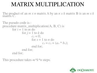
2.3 Matrix Multiplication. Background Example. We return to our Sweatshirt store example: We wish to find the value of the inventory by size Smalls - $10, Med - $11, Large - $12, XL - $13. How would we set up the mult. to do this?. Matrix Multiplication Algorithm.

E N D
Background Example • We return to our Sweatshirt store example: • We wish to find the value of the inventory by size • Smalls - $10, Med - $11, Large - $12, XL - $13 • How would we set up the mult. to do this?
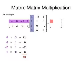
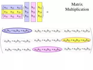
Matrix Multiplication Algorithm • The mtx mult algorithm is defined to do just that: • (i,j): multiply entries in row i of first mtx by the corresponding entries in col j of second mtx, and then add terms. • Note that this is the dot product of row i and col j
A few things to note • Given the way that the algorithm is defined, what must be true about the dimensions of the matrices in order for multiplication to work? • # of entries in each row of first matrix must equal # of entries in each column of second matrix • (i.e. number of columns of first matrix must equal the number of rows of second matrix) • So if multiplying matrices of following order: (a x b) x (c x d), b = c • Note: order of solution mtx is: a x d
Example • Given matrices A and B, find the results of the following if possible: • A2 • B2 • AB • BA
Example#2 • Given the matrices A and B, find AB and BA: • B is the identity matrix, I3, since AB = BA = A • The identity is always a square matrix with 1’s on the main diagonal and 0’s elsewhere. • I is only the identity for a matrix of the same size.
Properties of Mtx Multiplication • IA = A, BI = B • A(BC) = (AB)C • A(B+C) = AB + AC, A(B-C) = AB - AC • (B+C)A = BA + CA, (B - C)A = BA - CA • k(AB) = (kA)B = A(kB) • (AB)T = BTAT • Note: commutativity does not hold (AB ≠ BA in most cases). • Therefore the order of the factors in a product of matrices makes a difference!
Helpful Notation • To help us prove the properties, it is useful to understand the following notation for matrix multiplication. • A = [aij] is m x n, B = [bij] is n x p • ith row of A is [ ai1 ai2 …… ain] • jth column of B is:---------------------> • ij entry of prod mtx is dot prod of row i of A and col j of B:
Proving Property 3 (also in book) • Property 3: A(B + C) = AB + AC • A is m x n, B is n x p, C is n x p • B + C = [bij + cij] • This is just the (i,j) entry of AB + the (i,j) entry of AC • Therefore A(B + C) = AB + AC
Matrix form of linear system • Try to write the following system as a single matrix equation: • A is coefficient mtx, X is solution mtx, B is constant mtx
Precursor to Theorem 2 • If X1 is a sol’n to AX=B and X0 is a sol’n to the related homogeneous system AX = 0, then: • X1 + X0 is a solution to AX = B: • Theorem 2 is a converse of this.
Theorem 2 • If X1 is a sol’n to AX=B, then every solution, X2, to AX=B is of the form: • X2 = X1 + X0 where X0 is a solution to the associated homogeneous system AX=0.
Proof of Theorem 2 • If X2 and X1 are both sol’ns to AX=B, • So AX1 = B and AX2 = B: • say X0 = X2 - X1 so X2 = X0+X1 • AX0 = A(X2 - X1) = AX2 - AX1= B - B = 0 • Therefore, X0 is a solution to the associated homogeous system AX = 0.
Example • Express every solution to the following system as the sum of a specific solution plus a solution to the associated homogeneous system.
Solution • If we take t=0, we get a specific solution, X1 • Therefore, if t≠0, the solution, X2 = X1 + X0 where X0 is a solution to the associated homogeneous stm: AX = 0 • So, gives all sol’ns to assoc. hom. System • (Show)
Example • Find row 3 and column 2 of AB. • In many situations, it is helpful to write a matrix as a column of rows or as a row of columns:
Simplifying Notation • So then we can use the following notation in mtx mult:
A further simplification • We can partition a matrix into smaller blocks:
Continuing the Example • We need to make sure that the way we partition the matrices allows us to multiply matrices which match up appropriately by dimension. (show)
Another Block Multiplication Ex. • Go through ex. 11 with finding powers of mtx: • Find A8
Example continued • This was convenient since we have a 0 matrix • This was convenient since we had a diagonal matrix
Other topics in homework • Trace: sum of elements on main diagonal of square mtx • Idempotent: square mtx,P, is idempotent if P2 = P