Download

1 / 41
420 likes | 718 Views
Greedy Algorithms Spanning Trees. Chapter 16, 23. What makes a greedy algorithm?. Feasible Has to satisfy the problem’s constraints Locally Optimal The greedy part Has to make the best local choice among all feasible choices available on that step

E N D
Greedy AlgorithmsSpanning Trees Chapter 16, 23
What makes a greedy algorithm? • Feasible • Has to satisfy the problem’s constraints • Locally Optimal • The greedy part • Has to make the best local choice among all feasible choices available on that step • If this local choice results in a global optimum then the problem has optimal substructure • Irrevocable • Once a choice is made it can’t be un-done on subsequent steps of the algorithm • Simple examples: • Playing chess by making best move without lookahead • Giving fewest number of coins as change • Simple and appealing, but don’t always give the best solution
Activity Selection Problem • Problem: Schedule an exclusive resource in competition with other entities. For example, scheduling the use of a room (only one entity can use it at a time) when several groups want to use it. Or, renting out some piece of equipment to different people. • Definition: Set S={1,2, … n} of activities. Each activity has a start time si and a finish time fj, where si <fj. Activities i and j are compatible if they do not overlap. The activity selection problem is to select a maximum-size set of mutually compatible activities.
Greedy Activity Selection • Just march through each activity by finish time and schedule it if possible:
Activity Selection Example Schedule job 1, then try rest: (end up with 1, 4, 8): Runtime?
Greedy vs. Dynamic? • Greedy algorithms and dynamic programming are similar; both generally work under the same circumstances although dynamic programming solves subproblems first. • Often both may be used to solve a problem although this is not always the case. • Consider the 0-1 knapsack problem. A thief is robbing a store that has items 1..n. Each item is worth v[i] dollars and weighs w[i] pounds. The thief wants to take the most amount of loot but his knapsack can only hold weight W. What items should he take? • Greedy algorithm: Take as much of the most valuable item first. Does not necessarily give optimal value!
Fractional Knapsack Problem • Consider the fractional knapsack problem. This time the thief can take any fraction of the objects. For example, the gold may be gold dust instead of gold bars. In this case, it will behoove the thief to take as much of the most valuable item per weight (value/weight) he can carry, then as much of the next valuable item, until he can carry no more weight. • Moral • Greedy algorithm sometimes gives the optimal solution, sometimes not, depending on the problem. • Dynamic programming, when applicable, will typically give optimal solutions, but are usually trickier to come up with and sometimes trickier to implement.
Spanning Tree • Definition • A spanning tree of a graph G is a tree (acyclic) that connects all the vertices of G once • i.e. the tree “spans” every vertex in G • A Minimum Spanning Tree (MST) is a spanning tree on a weighted graph that has the minimum total weight Where might this be useful? Can also be used to approximate some NP-Complete problems
Sample MST • Which links to make this a MST? Optimal substructure: A subtree of the MST must in turn be a MST of the nodes that it spans.
MST Claim • Claim: Say that M is a MST • If we remove any edge (u,v) from M then this results in two trees, T1 and T2. • T1 is a MST of its subgraph while T2 is a MST of its subgraph. • Then the MST of the entire graph is T1 + T2 + the smallest edge between T1 and T2 • If some other edge was used, we wouldn’t have the minimum spanning tree overall
Greedy Algorithm • We can use a greedy algorithm to find the MST. • Two common algorithms • Kruskal • Prim
Kruskal’s MST Algorithm • Idea: Greedily construct the MST • Go through the list of edges and make a forest that is a MST • At each vertex, sort the edges • Edges with smallest weights examined and possibly added to MST before edges with higher weights • Edges added must be “safe edges” that do not ruin the tree property.
Kruskal’s Example • A={ }, Make each element its own set. {a} {b} {c} {d} {e} {f} {g} {h} • Sort edges. • Look at smallest edge first: {c} and {f} not in same set, add it to A, union together. • Now get {a} {b} {c f} {d} {e} {g} {h}
Kruskal Example Keep going, checking next smallest edge. Had: {a} {b} {c f} {d} {e} {g} {h} {e} ≠ {h}, add edge. Now get {a} {b} {c f} {d} {e h} {g}
Kruskal Example Keep going, checking next smallest edge. Had: {a} {b} {c f} {d} {e h} {g} {a} ≠ {c f}, add edge. Now get {b} {a c f} {d} {e h} {g}
Kruskal’s Example Keep going, checking next smallest edge. Had {b} {a c f} {d} {e h} {g} {b} {a c f}, add edge. Now get {a b c f} {d} {e h} {g}
Kruskal’s Example Keep going, checking next smallest edge. Had {a b c f} {d} {e h} {g} {a b c f} = {a b c f}, dont add it!
Kruskal’s Example Keep going, checking next smallest edge. Had {a b c f} {d} {e h} {g} {a b c f} = {e h}, add it. Now get {a b c f e h} {d}{g}
Kruskal’s Example Keep going, checking next smallest edge. Had {a b c f e h} {d}{g} {d} {a b c e f h}, add it. Now get {a b c d e f h} {g}
Kruskal’s Example Keep going, check next two smallest edges. Had {a b c d e f h} {g} {a b c d e f h} = {a b c d e f h}, don’t add it. a 6 4 9 5 b c d 14 2 10 e f g 15 3 8 h
Kruskal’s Example Do add the last one: Had {a b c d e f h} {g}
Runtime of Kruskal’s Algo • Runtime depends upon time to union set, find set, make set • Simple set implementation: number each vertex and use an array • Use an array member[] : member[i] is a number j such that the ith vertex is a member of the jth set. • Example member[1,4,1,2,2] indicates the sets S1={1,3}, S2={4,5} and S4={2}; i.e. position in the array gives the set number. Idea similar to counting sort, up to number of edge members.
Set Operations 1 2 3 • Given the Member array • Make-Set(v) member[v] = v Make-Set runs in constant running time for a single set. • Find-Set(v) Return member[v] Find-Set runs in constant time. • Union(u,v) for i=1 to n do if member[i] = u then member[i]=v Scan through the member array and update old members to be the new set. Running time O(n), length of member array. member = [1,2,3] ; {1} {2} {3} find-set(2) = 2 Union(2,3) member = [1,3,3] ; {1} {2 3}
Overall Runtime O(V) O(ElgE) – using heapsort O(E) O(1) O(V) Total runtime: O(V)+O(ElgE)+O(E*(1+V)) = O(E*V) Book describes a version using disjoint sets that runs in O(E*lgE) time
Prim’s MST Algorithm • Also greedy, like Kruskal’s • Will find a MST but may differ from Prim’s if multiple MST’s are possible
Prim’s Algorithm Get spanning tree by connecting nodes with their parents:
Runtime for Prim’s Algorithm O(V) if using a heap O(lgV) if using a heap O(V) O(E) over entire while(Q<>NIL) loop O(lgV) to update if using a heap! The inner loop takes O(E lg V) for the heap update inside the O(E) loop. This is over all executions, so it is not multiplied by O(V) for the while loop (this is included in the O(E) runtime through all edges. The Extract-Min requires O(V lg V) time. O(lg V) for the Extract-Min and O(V) for the while loop. Total runtime is then O(V lg V) + O(E lg V) which is O(E lg V) in a connected graph (a connected graph will always have at least V-1 edges).
Prim’s Algorithm – Linear Array for Q • What if we use a simple linear array for the queue instead of a heap? • Use the index as the vertex number • Contents of array as the distance value • E.g. Val[10 5 8 3 … ] Par[6 4 2 7 …] Says that vertex 1 has key = 10, vertex 2 has key = 5, etc. Use special value for infinity or if vertex removed from the queue Says that vertex 1 has parent node 6, vertex 2 has parent node 4, etc. Building Queue: O(n) time to create arrays Extract min: O(n) time to scan through the array Update key: O(1) time
Runtime for Prim’s Algorithm with Queue as Array O(V) to initialize array O(V) to search array O(V) O(E) over entire while(Q<>NIL) loop O(1) direct access via array index The inner loop takes O(E ) over all iterations of the outer loop. It is not multiplied by O(V) for the while loop. The Extract-Min requires O(V ) time. This is O(V2) over the while loop. Total runtime is then O(V2) + O(E) which is O(V2) Using a heap our runtime was O(E lg V). Which is worse? Which is worse for a fully connected graph?
Approximations for Hard Problems • Greedy algorithms are commonly used to find approximations for NP-Complete problems • Use a heuristic to drive the greedy selection • Heuristic: A common-sense rule that approximates moves toward the optimal solution • If our problem is to minimize a function f where • f(s*) is the value of the exact solution; global minimum • f(sa) is the value of our approximate solution • Then we want to minimize the ratio: • f(sa) / f(s*) such that this approaches 1 • Opposite if maximizing a function
Example: Traveling Salesman Problem • Cheap greedy solution to the TSP: • Choose an arbitrary city as the start • Visit the nearest unvisited city; repeat until all cities have been visited • Return to the starting city • Example graph: Starting at a: a->b->c->d->a Total = 10 Optimal: 8 a->b->d->c->a r(sa) = 10/8 = 1.25 1 a b 3 3 6 2 d c 1 Is this a good approach? What if a->d = 999999?
Greedy TSP • Our greedy approach is not so bad if the graph adheres to Euclidean geometry • Triangle inequality • d[i,j] ≤ d[i,k] + d[k,j] for any triple cities i,j,k • Symmetry • d[i,j] = d[j,i] for any pair of cities i,j • In our previous example, we couldn’t have a one-way edge to a city of 999999 where all the other edges are smaller (if a city is far away, forced to visit it some way) • It has been proven for Euclidean instances the nearest neighbor algorithm: • f(sa) / f(s*) ≤ (lg n + 1) / 2 n ≥ 2 cities
Minimum Spanning Tree Approximation • We can use a MST to get a better approximation to the TSP problem • This is called a twice-around-the-tree algorithm • We construct a MST and “fix” it up so that it makes a valid tour • Construct a MST of the graph corresponding to the TSP problem • Starting at an arbitrary vertex, perform a DFS walk around the MST recording the vertices passed by • Scan the list of vertices from the previous step and eliminate all repeat occurrences except the starting one. The vertices remaining will form a Hamiltonian circuit that is the output of the algorithm.
MST Approximation to TSP • Example graph: 12 a e a e 9 9 4 4 7 7 8 b d b d 8 8 6 6 12 12 c c MST: ab, bc, bd, de Walk: a, b, c, b, d, e, d, b, a a, b, c, d, e, a
MST Approximation • Runtime: polynomial (Kruskal/Prim) • Claim: • f(sa) < 2f(s*) • Length of the approximation solution at most twice the length of the optimal • Since removing any edge from s* yields a spanning tree T of weight w(T) that must be ≥ w(T*), the weight of the graph’s MST, we have: • f(s*) > w(T) ≥ w(T*) • 2f(s*) > 2w(T*) • The walk of the MST tree we used to generate the approximate solution traversed the MST at most twice, so: • 2w(T*) > f(sa) • Giving: • 2f(s*) > 2w(T*) > f(sa) • 2f(s*) > f(sa)