Download
1 / 7
70 likes | 179 Views
Bunch monitor signal integration. 13/12/13. Intro. P arallel bunch monitor (located after injection foil) Assume i ntegral of each peak proportional to bunch charge. Figures from Suzie’s presentation 13/11/13. H- beam injected. H+ beam circulating. Signal preprocessing.

E N D
Bunch monitor signal integration 13/12/13
Intro • Parallel bunch monitor (located after injection foil) • Assume integral of each peak proportional to bunch charge. Figures from Suzie’s presentation 13/11/13 H- beam injected H+ beam circulating
Signal preprocessing • Use Shinji’s peak finding algorithm to find set of tpeak • For every peak, isolate the signal for that turn, Seems tpeak – 30ns < t < tpeak + 50 ns is reasonable. • Remove slow variation (slope) in signal by subtracting from each point a line that passes through the minima on both sides.
Prepared signals First 20 turns First 81 turns in 10 turn steps
Area calculation methods • FWHM * width • Integrate under curve by quadrature (scipy.interpolate.quadrature • FWHM times indicated by dashed lines. • Asymmetric bunch broadending
Example result 1 (data from 1/11/13) • File: ~SortByDate/2013/11/13/1/?.csv (must check) • Area decreases for the first few turns. Plateau for some time and then drops again • Fit width vs turns in linear region to obtain dp (here we assume dp is fixed). Phase slip η from Zgoubi model at injection momentum. • Head-meets-tail debunchtime from dp calculation = 38 turns
Example result 2 (data from 1/11/13) • File: ~SortByDate/2013/11/13/1/double090.csv • No decrease in area for first few turns in this case • Debunchtime from dp calculation = 32 turns • Hints of rebunchingin data? Signal is weak, could be in the noise.