Download
1 / 37
370 likes | 551 Views
PARALLEL RANDOM NUMBER GENERATION. Ahmet Duran CISC 879. Outline. Random Numbers Why To Prefer Pseudo- Random Numbers Application Areas The Linear Congruential Generators Period of Linear Congruential Sequence Approaches to the Generation of Random Numbers on Parallel Computers

E N D
PARALLEL RANDOM NUMBER GENERATION Ahmet Duran CISC 879
Outline • Random Numbers • Why To Prefer Pseudo- Random Numbers • Application Areas • The Linear Congruential Generators • Period of Linear Congruential Sequence • Approaches to the Generation of Random Numbers on Parallel Computers • Centralized • Replicated • Distributed
Outline • Some Tests For Random Number Generators • Testing Parallel Random Number Generators • SPRNG (Scalable Library for Pseudorandom Number Generation)
Random Numbers • Well-known sequential techniques exist for generating, in a deterministic fashion, • The number sequences are largely indistinguishable from true random sequences • The deterministic nature is important because it provides for reproducibility in computations. • Efficiency is needed by preserving randomness and reproducibility
Random Numbers • Consider the following experiment to verify the randomness of an infinite sequence of integers in [1,d]. • Suppose we let you view as many numbers from the sequence as you wished to. • You should then guess any other number in the sequence. • If the likelihood of your guess being correct is greater than 1/d, then the sequence is not random. • In practice, to estimate the winning probabilities we must play this guessing game several times.
Why To Prefer Pseudo- Random Numbers • True random numbers are rarely used in computing because: • difficult to generate reliably • the lack of reproducibility would make the validation of programs that use them extremely difficult • Computers use pseudo-random numbers: • finite sequences generated by a deterministic process • but indistinguishable, by some set of statistical tests, from a random sequence.
Application Areas • Simulation: When we simulate natural phenomena, random numbers are required to make things realistic. For example: Operations research (where people come into airport at random intervals.) • Sampling: It is often impractical to examine all possible cases, but a random sample will provide insight into what constitutes "typical" behaviour. • Computer Programming: Random values make good source of data for testing the effectiveness of computer algorithms.
Application Areas • Numerical Analysis • Decision Making: There are reports that many executives make their decisions by flipping a coin or by throwing darts, etc. • Aesthetics: A little bit randomness makes computer-generated graphics and music seem more lively. • Recreation: "Monte Carlo method", a general term used to describe any algorithm that employs random numbers.
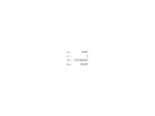
The Linear Congruential Generators • Generator is a function, when applied to a number, yields the next number in the sequence. For example, • X_k+1 = (a * X_k + c) mod m where X_k is the k th element of the sequence and X_0, a, c , and m define the generator. • As numbers are taken from a finite set (for example, integers between 1 and 2^31), any generator will eventually repeat itself.
The Linear Congruential Generators • The length of the repeated cycle is called the period of the generator. • A good generator is one with a long period and no discernible correlation between elements of the sequence. • Example: X_k+1 = (3 * X_k + 4) mod 8 E = {1, 7, 1, 7, …} is bad.
Period of Linear Congruential Sequence • Theorem: The linear congruential sequence has period m if and only if • c is relatively prime to m; • b = a - 1 is a multiple of p, for every prime p dividing m; • b is a multiple of 4, if m is a multiple of 4. • Example: X_k+1 = (7 * X_k + 5) mod 18 E = {1, 12, 17, 16, 9, 14, 13, 6, 11, 10, 3, 8, 7, 0, 5, 4, 15, 2, 1,…}
Approaches to the Generation of Random Numbers on Parallel Computers • Centralized • Replicated • Distributed
Centralized Approach • A sequential generator is encapsulated in a task from which other tasks request random numbers. • Advantages: • Avoids the problem of generating multiple independent random sequences • Disadvantages: • Unlikely to provide good performance • Makes reproducibility hard to achieve: the response to a request depends on when it arrives at the generator, and the result computed by a program can vary from one run to the next.
Replicated Approach • Multiple instances of the same generator are created (for example, one per task). Each generator uses either the same seed or a unique seed, derived, for example, from a task identifier. • Advantages: • Efficiency • Ease of implementation • Disadvantages: • Not guaranteed to be independent and, can suffer from serious correlation problems.
Distributed Approach • Responsibility for generating a single sequence is partitioned among many generators, which can then be parcelled out to different tasks. • Advantages: • The analysis of the statistical properties of the distributed generator is simplified because the generators are all derived from a single generator • Efficiency • Disadvantages: • Difficult to implement on parallel computers
Distributed Approaches • The techniques described here are based on an adaptation of the linear congruential algorithm called the random tree method. • This facility is particularly valuable in computations that create and destroy tasks dynamically during program execution. • The Random Tree Method • The Leapfrog Method • Modified Leapfrog
L R0 R1 R2 The Random Tree Method • The random tree method employs two linear congruential generators, L and R , that differ only in the values used for a . • L_k+1 = a_L L_k mod m • R_k+1 = a_R R_k mod m
Application of the left generator L to a seed generates one random sequence; application of the right generator R to the same seed generates a different sequence. • By applying the right generator to elements of the left generator's sequence (or vice versa), a tree of random numbers can be generated. • By convention, the right generator R is used to generate random values for use in computation, while the left generator L is applied to values computed by R to obtain the starting points R0, R1 , etc., for new right sequences.
Random Tree Method • Advantages: • Useful to generate new random sequences in a reproducible and noncentralized fashion. This is valuable, in applications in which new tasks and hence new random generators must be created dynamically. • Disadvantages: • There is no guarantee that different right sequences will not overlap. If two starting points happen to be close to each other, the two right sequences that are generated will be highly correlated.
The Leapfrog Method • A variant of the random tree method • Used to generate sequences that can be guaranteed not to overlap for a certain period. • Useful where a program requires a fixed number of generators. (For example, one generator for each task ).
R1 R0 L_0 L_1 L_2 L_3 L_4 L_5 L_6 L_7 L_8 R2 Figure: The leapfrog method with n=3. Each of the right generators selects a disjoint subsequence of the sequence constructed by the left generator’s sequence.
Let n be the number of sequences required. Then we define a_L and a_R as a and a^n, respectively, • L_k+1 = a L_k mod m • R_k+1 = a^n R_k mod m • Create n different right generators R0 .. Rn-1 by taking the first n elements of L as their starting values. • The name “leapfrog method” refers that the i th sequence Ri consists of L_i and every n th subsequent element of the sequence generated by L. • As the method partitions the elements of L, each subsequence has a period of at least P/n, where P is the period of L. • The n subsequences are disjoint for their first P/n elements.
The generator for the r th subsequence, Rr , is defined by a^n and Rr_0 = L_r. • First, compute a^r and a^n • Then, compute members of the sequence Rr as follows, to obtain n generators, each defined by a triple (Rr_0, a^n, m) , for 0 <= r < n . • Rr_0 = (a^r L_0) mod m • Rr_i+1 = (a^n Rr_I) mod m
Modified Leapfrog • A variant of the leapfrog method • Used in situations, where we know the maximum number, n , of random values needed in a subsequence but not the number of subsequences required. • The role of L and R are reversed so that the elements of subsequence i are the contiguous elements • L_k+1 = a^n L_k mod m • R_k+1 = a R_k mod m • It is not a good idea to choose n as a power of two, as this can lead to serious long-term correlations.
R0 R1 R2 … L_0 L_1 L_2 L_3 L_4 L_5 L_6 L_7 L_8 Figure: Modified leapfrog with n=3 . Each subsequence contains three contiguous numbers from the main sequence.
Some Tests For Random Number Generators • The basic idea behind the statistical tests is that the rabdom number streams obtained from a generator should have the properties of a random sample drawn from the uniform distribution. • Tests are designed so that the expected value of some test statistic is known for uniform distribution. • The empirically generated random number stream is then subject to the same test, and the statistic obtained is compared against the expected value.
Frequency Test • The focus of the test is the proportion of zeroes and ones for the entire sequence. • Example: • (input) E=1100100100001111110110101010001000100001011010001100001000110100110001001100011001100010100010111000 • (input) n = 100 • (output) P-value = 0.109599 • (conclusion) Since P-value >= 0.01, accept the sequence as random.
Runs Test • A run is an uninterrupted sequence of identical bits. • The focus of this test is the total number of runs in the sequence. • A run of length k consists of exactly k identical bits and is bounded before and after with a bit of the opposite value. • The purpose of the runs test is to determine whether the number of runs of ones and zeros of various lengths is as expected for a random sequence. • Determines whether the oscillation between such zeros and ones is too fast or too slow.
Runs Test • A fast oscillation occurs when there are a lot of changes, e.g., 010101010 oscillates with every bit. • (input) E = 1100100100001111110110101010001000100001011010001100001000110100110001001100011001100010100010111000 • (input) n = 100 • (output) P-value = 0.500798 • (conclusion) Since P-value >= 0.01, accept the sequence as random.
Testing Parallel Random Number Generators • A good parallel random number generator must be a good sequential generator. • Sequential tests check for correlations within a stream, while parallel tests check for correlations between different streams.
Testing Parallel Random Number Generators • Exponential sums • Parallel spectral test • Interleaved tests • Fourier transform test • Blocking test
Fourier Transform Test • Fill a two dimensional array with random numbers. Each row of the array is filled with random numbers from a different stream. • Calculate the Fourier coefficients and compare with the expected values. • This test is repeated several times and check if there are particular coefficients that are repeatedly “bad”.
Blocking Test • Use the fact that the sum of independent variables asymptotically approaches the normal distribution to test for the independence of random number streams. • Add random numbers from several stream and form a sum. • Generate several such sums and check if their distribution is normal.
SPRNG • A “Scalable Library for Pseudorandom Number Generation”, • Designed to use parametrized pseudorandom number generators to provide random number streams to parallel processes. • Includes • Several, qualitatively distinct, well tested, scalable RNGs • Initialization without interprocessor communication • Reproducibility by using the parameters to index the streams
Reproducibility controlled by a single “global” seed • Minimization of interprocessor correlation with the included generators • A uniform C, C++, Fortran and MPI interface • Extensibility • An integrated test suite.
Refences: • Introduction to Parallel RNGs http://sprng.cs.fsu.edu/Version1.0/paper/index.html • Random Number Generation on Parallel Computer Systems http://www.npac.syr.edu/projects/reu/reu94/cstoner/proposal/proposal.html • SPRNG (Scalable Parallel Pseudo Random Number Generators Library) http://sprng.cs.fsu.edu/
References (continued) • A. Srinivasan, D. Ceperley and M. Mascagni, Testing Parallel Random Number Generators http://sprng.cs.fsu.edu/links.html • M. Mascagni, D. Ceperley and A. Srinivasan, SPRNG: A Scalable Library for Pseudorandom Number Generation http://sprng.cs.fsu.edu/links.html • Ian Foster, Designing and Building Parallel Programs • D. E. Knuth, The Art of Computer Programming, Volume 2, Seminumerical Algorithms, Third Edition