Download
1 / 18
250 likes | 635 Views
Derivation and Use of Reflection Coefficient. Transmission Line Model. I F. I T. + V F _. + V T _. Z S. Z 0. Z T. +_. V S. x. Forward Power (positive x direction): V F = I F Z 0 Matched source of power. Assume Z S = Z 0 = R + j 0

E N D
Transmission Line Model IF IT + VF _ + VT _ ZS Z0 ZT +_ VS x • Forward Power (positive x direction): VF = IFZ0 • Matched source of power. Assume ZS = Z0 = R + j0 • Terminating impedance: ZT = RT + jXT ; VT = ITZT • What’s wrong with this picture?
Terminating Condition ( x = 0 ) IF IT + VF _ + VT _ ZS Z0 ZT +_ VS x At x = 0, IF(0) = IT and VF(0) = VTif and only ifZT = Z0 !! But . . . ZT can be ANYTHING!!! Therefore, there must exist additional voltages and currents in the transmission line such that the Total Line Current and Total Line Voltage at x = 0 satisfy continuity: IL(0) = IT = IF(0) + [?] and VL(0) = VT = VF(0) + [?]
The mystery terms in the brackets must also correspond to voltages and currents associated with the transmission of power in the line. We have already accounted for power traveling in the positive x direction (forward power). The mystery terms in the brackets must therefore correspond to voltages and currents associated with the transmission of power in the opposite (negative x) direction. This represents the portion of forward power not absorbed by the terminating load, and “reflected” back toward the source. The voltage and current associated with the reflected power must still obey: VR = IRZ0 IR + VR _ Z0 x
Now we do the Math! IL = (IF – IR) IT + VL = (VF + VR) _ + VT _ ZS Z0 ZT +_ VS x The total voltage and current in the transmission line is the superposition (sum) of the voltages and currents associated with the forward and reflected power. The continuity condition at the termination (x = 0) is:
(Continuing) …by inspection: Define Normalized Impedance: Define Reflection Coefficient: Rewrite the above, and define GT = G(0) QED:
Recap . . . • Based on fundamental principles, we have determined that the voltage and current that we would measure on a transmission line is the superposition of two sets of voltages and currents, corresponding to power flowing in both directions. • We have defined the concept of normalized impedance. • We have defined the concept of reflection coefficient, and determined how to compute it’s value at the termination point of a transmission line, given the terminating impedance.
Observations • The forgoing results are independent of the mathematical form of the voltage function. It can be any complex function of time and position. However, having invoked the concept of Impedance, a sinusoidal (complex exponential) function of time is implied. • Our definition of reflection coefficient constrains its magnitude to unity or less, thus it may be represented by a vector (point) on the complex plane lying within or on the “Unit Circle”.
ZL: Line Impedance The quintessential computation when working with transmission lines is the determination of the Impedance (or Admittance) presented by a line of length l terminated by ZT. By definition, Line Impedance is the ratio of total Line Voltage to total Line Current: IL(x = -l) IT + VL(x = -l) _ + VT _ Z0 ZT ZL(x = -l) x (x = -l) (x = 0)
Line Reflection Coefficient I order to determine Reflection coefficient at any point, x, along the line, we will incorporate the forms for the Forward and Reflected Voltage waveforms determined previously: At the termination point (x = 0 ), Substituting, We see from the above that the reflection coefficient, when considered as a Polar (not Cartesian) complex vector, is “well behaved”, in the sense that it is a vector of fixed magnitude < 1, with only its complex phase angle affected by the distance from the line termination to the point of interest.
Conceptual Solution to the Fundamental Problem Find the impedance presented by a transmission line having characteristic impedance Z0 and length l, when terminated with impedance ZT. Step 1 Determine Reflection Coefficient at the Termination. Step 2 Rotate the Reflection Coefficient Vector by an angle corresponding to the “electrical length” of the line. Step 3 Determine Line Impedance from the rotated Reflection Coefficient vector.
The Smith Chart The Smith Chart is a graphical tool which performs the computations of steps 1 and 3 graphically. Early Smith Charts were scaled to a specific transmission line characteristic impedance. Now, all Smith charts are normalized to a characteristic impedance of 1 ohm, so the practical procedure using a smith chart has five steps: Normalize Terminating Impedance Draw Reflection Coefficient vector corresponding to Normalized Terminating Impedance. (Old step 1) Rotate the Reflection Coefficient Vector by an angle corresponding to the “electrical length” of the line. (Old step 2) Read the Normalized Line Impedance from the tip of the rotated Reflection Coefficient vector. (Old step 3) De-normalize the Line Impedance.
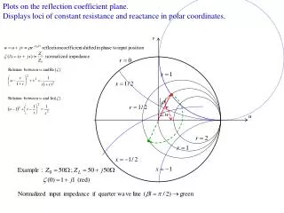
How does it work? Consider the fundamental equation relating Impedance to Reflection coefficient: Z = R +jX If we take every possible value of Z from the complex Z Plane (RHS), and plot the Reflection Coefficient according to the equation above, you get every possible point inside (or on) the unit circle.
Reflection Coefficient: Special Cases Short Circuit Since r = 1, the magnitude of the forward and reflected voltage waves are equal. Since their phase difference is p, they will sum to zero volts at the termination point. Open Circuit Since r = 1, the magnitude of the forward and reflected voltage waves are equal. Since their phase difference is 0, they will sum to a voltage maximum at the termination point.
Shorted Quarter Wave Line Consider a line, terminated with a short circuit, having length l such that: -2bl = -p, or l =(p/2)/b. Recall that b = w/vp = 2pf/vp = 2p/l. Thus l = l/4 (quarter wave). Z0 GT Gl x (x = -l = -l/4) (x = 0) We see that a distance on the transmission line corresponding to one quarter wavelength represents a rotation of p radians of the reflection coefficient vector. A short circuit is “transformed” to an open circuit, and vice versa.
Standing Wave Example + VL _ + VT _ Consider a line terminated with impedance ZT = 3Z0 . We have ZS ZT = 3 Z0 Z0 +_ VS This means that the amplitude of the reflected wave is half that of the forward wave. Since the phase difference is zero at x = 0, the amplitudes add, yielding a voltage maximum: |VL(max)| = (1+r)| VF | = 1.5 |VF| One quarter wave distant from the termination, x = -l/4, the reflection coefficient vector will have rotated by p radians, the reflected wave will be exactly out of phase with the forward wave and the amplitudes will subtract, yielding a voltage minimum: |VL(min)| = (1-r)| VF | = 0.5 |VF| x At x = -l/2 (an additional quarter wave away from the load), the phase difference will be 2p (or zero), and there will be another voltage maximum. This variation in amplitude of VL as we move along the line is called a standing wave, and is characterized by the “Standing Wave Ratio” (SWR), which is the ratio of Voltage maximum to voltage minimum:
r and SWR If the phase angle of G is 0 (positive real axis ), then Thus the constant r circle crosses the positive real axis where
Standing Wave Measurements Consider a 50 ohm line (eR = 1.69) terminated with an unknown impedance ZT . We measure a voltage maximum of 6.5 VAC at a point 0.3 m from the termination, and a voltage minimum of 2.7 VAC at a point 1.1 meters from the termination. Since voltage max/min are always separated by l/4, l = 4(1.1 - 0.3) = 3.2 m. + VL(min) _ + VL(max) _ ZS ZT = ? Z0 +_ VS The “electrical” distance (bl) from the termination to the voltage maximum is 0.3/3.2 = 0.09375 l = 33.75o = 0.59R x If eR = 1.69, vp= ceR(-1/2) = c/1.3 f = vp / l = c/(1.3)(3.2 m)= 72.116 Mhz -1.1 -0.3 0 67.5O r = 0.414 GT G@Vmin G@Vmax