Download
1 / 32
380 likes | 699 Views
ENGR 691, Fall Semester 2010-2011 Special Topic on Sedimentation Engineering Section 73 Coastal Sedimentation. Yan Ding, Ph.D.

E N D
ENGR 691, Fall Semester 2010-2011Special Topic on Sedimentation EngineeringSection 73Coastal Sedimentation Yan Ding, Ph.D. Research Assistant Professor, National Center for Computational Hydroscience and Engineering (NCCHE), The University of Mississippi, Old Chemistry 335, University, MS 38677 Phone: 915-8969 Email: ding@ncche.olemiss.edu
Outline • Introduction of morphodynamic processes driven by waves and currents in coasts, estuaries, and lakes • Initiation of motion for combined waves and currents • Bed forms in waves and in combined waves and currents • Bed roughness in combined waves and currents • Sediment transport in waves • Sediment transport in combined waves and currents • Transport of cohesive materials in coasts and estuaries • Mathematical models of morphodynamic processes driven by waves and currents • Introduction of a process-integrated modeling system (CCHE2D-Coast) in application to coastal sedimentation problems
Introduction • The transport of bed material particles by a flow of water can be in the form of bed-load and suspended load, depending on the size of the bed material particles and the flow conditions. The suspended load may also contain some wash load (usually, d<0.05mm), which is generally defined as that portion of the suspended load which is governed by the upstream supply rate and not by the composition and properties of the bed material. • The sediment transport in a steady uniform current is assumed to be equal to the transport capacity defined as the quantity of sediment that can be carried by the flow without net erosion or deposition, given sufficient availability of bed material (no amour layer). • Various types of formulae are available for predicting the bed-load and the suspended load transport (q). The formulae can be divided in five main groups as defined by the relevant hydraulic parameters: • Fluid velocity • Bed shear stress • Probabilistic particle movement • Bed form celerity • Energetics (stream power) :depth-averaged velocity m = 3 ~ 5 n ≈ 1.5 ucr: critical shear velocity τ: bed shear stress τcr: critical bed shear stress
Three Modes of Particle Motions • Three particle motions: • Rolling and sliding motion or both: • Saltation: • Suspended particle motion: Bed shear velocity just exceeds the critical value Bed shear velocity further increases Bed shear velocity exceeds the particle fall velocity
Bed-Load Transport Definition Bagnold’s definition (1956): In the bed-load transport, the successive contacts of the particles with the bed are strictly limited by the effect of gravity, while the suspended-load transport is defined as that in which the excess weight of the particles is supported by random successions of upward impulses imported by turbulent eddies. Einstein’s definition (1950): The bed-load transport is the transport if sediment particles in a thin layer of 2 particle diameters thick just above the bed by sliding, rolling, and sometimes by making jumps with a longitudinal distance of a few particle diameters. Bed-load transport = the transport of particles by rolling, sliding, and saltating Brigadier Ralph Alger Bagnold, OBE, FRS (3 April 1896 – 28 May 1990) was the founder and first commander of the British Army's Long Range Desert Group during World War II. Hans Albert Einstein (May 14, 1904 – July 26, 1973) was a professor at University of California, Berkeley. He was the second child, and the first son, of renowned physicist Albert Einstein (1879–1955) and his first wife, MilevaMarić (1875–1948).
Sediment Model Definitions Volumetric Bed-load transport: Cb = volumetric concentration in the bed-load layer ub = particle velocity (m/s) δb = thickness of bed-load layer (m) Suspended-load transport:
Issues for Calculating Sediment Transport Rate Bed-load Layer Thickness: Saltation height Particle Velocity Particle pick-up rate from the bed
Deterministic Bed-Load Transport Formulae Meyer-Peter Mueller (1948) Dimensionless bed-load transport rate: Particle mobility parameter: ks,c = effective bed roughness dm = mean particle diameter θcr = 0.047 Bagnold (1966) Van Rijn(1984a) Fig. 7.2.12
Suspended Load Transport z=h u(z) c(z) uc(z) ca z=a z=0 Ca = reference concentration or Van Rijn (1984) a = reference level: bed form height
Bed Material Suspension and Transport in Waves Wave motion over an erodible sand bed can generate a sediment suspension with relatively large sediment concentration in the near-bed region in the case of non-breaking waves. The key role of the breaking waves on the sediment concentration field in the coastal zone is obvious. The concentrations are maximum near the plunging point and decrease sharply on the both sides of the plunging area. The bed material is usually coarsest in the most energetic area and finer inside the surf zone and outside the surf zone. Wave-induced transport processes are related to the currents generated by waves. Net onshore transport is dominant in non-breaking wave conditions. Net offshore transport is dominant in breaking wave conditions. Fig. 8.1.1
Transport Processes in Breaking Waves (Surf Zone) • Mechanisms: • net backward (offshore) transport due to the generation of a net return flow (undertow) in the near-bed region in spilling and plunging breaking waves. • net forward (onshore) transport by asymmetrical wave motion in weakly spilling breaking waves. • longshore and offshore-directed transport due to the generation of large-scale circulation cells with longshore currents and offshore rip current. • gravity-induced transport (bed load) in downsloping direction
Current & Sediment Wave Breaking Line Longshore Sediment Transport Ocean City Beach looking north, Maryland Downloaded from: http://images.usace.army.mil/main.html Observations on natural beaches as well as in laboratory wave basins have confirmed that the longshore current is largely confined to the surf zone. This longshore current drives the shoreward movement of longshore sediment transport.
Computation of Sediment Transport Rates Induced by Waves • Two Approaches: • Sediment transport models representing both the instantaneous fluid velocity and concentration profile • Sediment transport formulae similar to the current-related bed-load formulae. 1. Sediment Transport Models (Local 1-D) This approach is useful when the phase difference between the instantaneous velocities and sediment concentrations at different elevations above the bed can not be neglected. Dividing the instantaneous velocity (U) and concentration (C) into two parts: and The net total time-averaged total transport rate can be expressed as: Not a ! qc qw + = the current-related part + the wave-related part Neglecting the horizontal convection, the horizontal diffusion and the vertical convection, the simplified concentration equation reads as: w= fall velocity; ε= mixing coefficient
Sediment Transport Formulae Since the major part of the sediment suspension in wave conditions is confined to a region close the bed (within 3 to 5 the ripple height or the sheet flow layer thickness), it seems reasonable to compute the wave-related sediment transport by a simple formula in analogy with the bed-load transport formulae applied in steady currents. A division between bed load and suspended load is only academic interest. The existing formulae are generally based on empirical concepts, as used in steady uniform flow, using experimental data of oscillating flow in wave tanks, wave tunnels, etc. Measures of sediment transport rates in waves: qw,half= the sediment transport rate in half a period of an oscillatory flow qw,net= the net sediment transport rate per wave cycle (period) In general, • Assumptions: • No phase differences between the instantaneous bed shear stress (τb,w) and the velocity outside the boundary layer (U) • No phase differences between instantaneous bed shear stresses and instantaneous transport rates
Instantaneous Total Sediment Transport Rate (Grant & Madsen, 1976) Total Sediment Transport Model (1) (m2/s) Instantaneous velocity vector near the bed Particle mobility parameter WS = particle fall velocity d50 = median particle diameter of bed material uc = near-bed current velocity UW = near-bed orbital velocity fw= friction factor f = angle between current direction and wave propagation direction
Total Sediment Transport Model (2) Time-averaged (over half a period) Total Sediment Transport Rate (Grant & Madsen, 1976) Other formulae Bailard-Bagnold (1981) : the instantaneous total transport rate (bed-load+suspended load) Sato-Horikawa (1986): the net transport rate based on wave tunnel experiments with regular asymmetric wave motion over a ripple sand bed Van Rijn (1989): asymmetric regular swell waves, asymmetric irregular wind waves, mean (weak) current in presence of waves, and bound long waves
Bed Material Suspension and Transport in Combined Waves and Currents • Currents in Coasts and Oceans: • tidal current • wind-induced currents • wave-induced currents (especially wave breaking) • vertical mixing due to bottom boundary turbulence • These current will result in additional upward transport of particles yielding larger concentrations in the upper layer. The basic mechanism is the entrainment of particles by the stirring wave action and the transport of the particles by the current motion. • The total sediment transport in combined waves and currents can be divided into: = current-related transport rate + wave-related transport rate qt,c: the transport of particles by the time-averaged current velocities qt,w: the transport of particles by the oscillating fluid motions (orbital velocities
Issues in Sediment Transport in Combined Waves and Currents • Non-breaking Waves: • Breaking Waves • Angle between wave and current: • wave-current interaction: following current and oppose current Return flow Wave direction current direction shoreline
Bed-load Transport (1:only current) • van Rijn’s model (Rijn, 1984) { qb = Volumetric bed-load transport rate Cb = Volumetric concentration δb = Thickness of bed load layer ub = Bed load particle velocity D* : Dimensional Particle paramter d50 : median particle diameter of bed material (m) /b,c :effective bed-shear stress due to combined current (N/m2) T: dimensionless bed-shear parameter
Bed-load Transport (2: wave+current) • Van Rijn’s model (Rijn, 1993) Time-averaged bed-load transport rate can be obtained by averaging the instantaneous values qb(t)over the whole wave period qb : instantaneous Volumetric bed-load transport rate (m2/s) D* : Dimensional Particle parameter d50 : median particle diameter of bed material (m) b,cr :critical bed-shear stress according to Shields (N/m2) /b,cw :grain-related instantaneous bed-shear stress due to combined current (N/m2) : fluid density (kg/m3) :calibration factor = 1-(Hs/h)0.5 , Hs: significant wave height (m)
Bed-load Transport due to Combined Current and Wave Instantaneous bed-load transport rate Satoh & Kabiling (1994) Shields Number yc = Critical Shield number ab = empirical coefficient (=1.0) Ub = near-bed current velocity
Van Rijn’s Sediment Transport Model: TRANSPOR Input Parameters: h = water depth VR= depth-averaged velocity vector of current uR = time-averaged and depth-averaged return flow velocity (- in offshore direction) ub = time-averaged near-bed velocity due to waves Hs = significant wave height Tp = peak wave period φ = angle between wave and current (deg) d50= median diameter of bed materials d90= 90% diameter of bed materials ds= representative diameter of suspended material ks,c=current-related bed roughness height ks,w=wave-related bed roughness height Te = water temperature (oC) SA = salinity Fig. Schematic illustration of current and wave directions
Van Rijn’s Sediment Transport Model: TRANSPOR TRANSPOR.for TRANSPOR.exe Appendix A in Van Rijn’s Book My version: cf_tanaka.for, cf_tanaka.exe Code: in my folder /TRANSPOR
Homework 4 (optional) (1) Using TRANSPOR sediment transport model and the following parameters, calculate sediment transport rates by wave and current. HD = WATER DEPTH [ M ] = 1.0000000 VR = MEAN VEL. IN CURRENT DIR. [ M/S ] = 0.200000 UR = MEAN VEL. IN WAVE DIR(-BACK) [ M/S ] = 0.4000000 UB = NEAR-BED VEL IN WAVE DIR(-BACK) [ M/S ]= 0.3000000 HS = SIGNIFICANT WAVE HEIGHT [ M ] = 0.5000 TP = PEAK WAVE PERIOD [ S ] = 4.50000 PHI = ANGLE CURRENT AND WAVES 0-360 [ DEG ] 60.0000000 D50 = MEDIAN PARTICLE SIZE OF BED [ M ] = 0.0002 D90 = 90 0/0 PARTICLE SIZE OF BED [ M ] = 0.0004 DSS = SUSPENDED SEDIMENT SIZE [ M ] = 0.00015 RC = CURRENT-RELATED ROUGHNESS [ M ] = 0.0200000 RW = WAVE-RELATED ROUGHNESS [ M ] = 0.0200000 TE = WATER TEMPERATURE [ CELSIUS ] = 20.0000000 SA = SALINITY OF FLUID [ PROMILLE ] = 35.0000000 (2) Input different wave heights, e.g. 0.5, 0.8, and 1.5 m, investigate the variations of sediment transport rate.
Longshore Sediment Transport by Wave Breaking Significant Wave Direction Supply of Sediment:small Sediment Rate: Eroded shoreline propagation of erosion 1 year 10 year 5 year Significant Wave Direction Sediment Rate: decrease Stabilization of Shoreline Beach
Shoreline Erosion Protection Protection of shoreline erosion by wave dissipating breakwaters and sand nourishments near the Fuji river mouth, Japan Protected by Coastal Structure: Artificial Headland
Ql Estimation of Longshore Sediment Rate- Energy Flux Method (CERC formula) (m3/s) K=empirical coefficient in the CERC Formula l = in-place sediment porosity Energy Flux = (ECg)b Hb : Wave Height at the breaker line (Cg)b : Wave group speed at the breaker line
Empirical Coefficient K- (Shore Protection Manual, 1984) K SPM 0.92 Komar & Inman (1970) 0.77 Takagi & Ding (2000) 0.06* *Nourished sand (gravel) + in-place sediment K=K(d)
Shoreline Evolution Model (Long-term)- One Line Model (Hanson & Kraus, 1989) • Assume the beach profile is displaced parallel to itself in the cross-shore direction - Parallel Contour Lines y= location of shoreline dc= offshore closure depth db=berm crest elevation q=line source or sink of sediment Fig. Elemental volume on equilibrium beach profile
Sketch of Seasonal Change between Two Headlands Incident wave in winter Incident wave in summer Maximum erosion 1km Shoreline in winter Shoreline in summer Variation of shoreline: seasonal wave height, wave direction, even daily data