Download
1 / 36
360 likes | 608 Views
GIS Applications in Civil Engineering Note #2 GIS Roots in Cartography. Xudong Jia, Ph.D., P.E. December, 2011. GIS Root in Cartography. GIS is a map-based information system.

E N D
GIS Applications in Civil Engineering Note #2 GIS Roots in Cartography Xudong Jia, Ph.D., P.E. December, 2011
GIS Root in Cartography • GIS is a map-based information system. • Cartography deals with maps. It is the art and science of map making, practiced by cartographers. Combining science, aesthetics, and technique, cartography builds on the premise that reality can be modeled in ways that communicate spatial information effectively. • A GIS map contains layers • Layers may contain features or surfaces • Features have shape and size • Surfaces have numeric values rather than shapes • Features have locations • Features can be displayed at different sizes
GIS Root in Cartography • Features are linked to information • Features have spatial relationships • New features can be created from areas of overlap
GIS Root in Cartography GIS Tools Provided by ESRI • ArcGIS Desktop • ArcReader • ArcView ArcMap, ArcCatalog • ArcEditor ArcMap, ArcCatalog;ArcEditor plus data creation and editing tools • ArcInfo ArcMap, ArcCatalog; ArcEditor plus more spatial analysis tools • Extensions ArcGIS 3D Analyst, ArcGIS Geostatistical Analyst ArcGIS Network Analyst, ArcGIS Schematics, ArcGIS Spatial Analyst, ArcGIS Survey Analyst , ArcGIS Tracking Analyst, Business Analyst Online Reports Add-In, and more
GIS Root in Cartography GIS Tools Provided by ESRI • Server GIS • ArcGIS Server • ArcGIS Server Extensions • ArcGIS for AutoCAD • ArcGIS Mapping for SharePoint • Online GIS • ArcGIS Online • ArcGIS Online Map Services • ArcGIS Online Task Services • Community Maps Program
GIS Root in Cartography GIS Tools Provided by ESRI • Mobile GIS • ArcGIS Mobile • ArcPad • Apps for Smartphones • Apps for IPhone • Online GIS • ArcGIS Online • ArcGIS Online Map Services • ArcGIS Online Task Services • Community Maps Program
GIS Root in Cartography GIS Tools Provided by ESRI • Developer Tools • ArcGIS Web Mapping—Flex, JavaScript, and Silverlight • Mobile API—ArcGIS for iOS • Tools for Java • Tools for .NET • Esri Developer Network (EDN) • ArcGIS Engine
GIS Root in Cartography What is on a map? A good map will have a legend or key which will show the user what different symbols mean. Without a north arrow and scale, it is difficult to determine the orientation and the size of a map. A neatline is the border of a map. It helps to define the edge of the map area and obviously keeps things looking "neat." Since the map is a flat representation of the curved surface of the earth, it needs projection. A map's title provides important clues about the cartographer's intentions and goals. Color appears so often on maps that we often take it for granted that mountains are brown and rivers are blue.
GIS Root in Cartography • Integration of GIS with Cartography needs to deal with: • Map and attribute information • Map scale and projections • Coordinate Systems
GIS Map and Attribute Information • GIS Geo-relational database model Vector map points, lines, or polygons Attribute Table Raster map Color Ramp • GIS Geodatabase model Vector map points, lines, or polygons Attribute Table Database Tables Database Table Database
Map Scale and Projections The shape of the earth How big is the earth? We need to calculate by how much to reduce the drawing of it to fit into the computer screen. (Map scale) What shape is the earth? The way we scale the map is not even worldwide due to the fact that the earth shape is not a perfect sphere. (Map scale and projection) How a feature is located on a map? A flat map and the simple pairs of numbers or coordinates be used to describe locations on the earth’s surface. (Map Projection)
Map Scale and Projections The shape of the earth
Map Scale and Projections The shape of the earth Ross Clarke in 1866: Semi-Major radius: 6,378,206.4 m Semi-Minor radius: 6,356,538.8 m Flattening: 1/294.9787 International Standard 1924: Semi-Major radius: 6,378,388 m Semi-Minor radius: ? m Flattening: 1/297 NAD 27 (North American Datum of 1927) (Clarke’s numbers)
Map Scale and Projections The shape of the earth GRS 80 (NAD 83) Semi-Major radius: 6,378137.0 m Semi-Minor radius: 6,356,752.314 140 m Flattening: 1/298.257 222 101 WGS 84 Semi-Major radius: 6,378,137.0m Semi-Minor radius: 6,356,752 314 245 m Flattening: 1/298.257 223 563
Map Scale and Projections The shape of the earth Geodesy (measuring the earth’s size, shape, and gravitational fields) mapped local variations from the ellipsoid to the geoid surface.
Map Scale and Projections All maps, whether on a sheet of paper or inside a computer, are reductions in size of the earth. Length of the Equator at Different Map Scale Scale Map Distance (m) Map Distance in feet 1:400,000,000 0.10002 0.328 (3.9 inches) 1:40,000,000 1.0002 3.28 1:10,000,000 4.0008 13.1 1:1,000,000 40.008 131 1:250,000 160.03 525 1:100,000 400.078 1,312 1:50,000 800.157 2,625 1:24,000 1,666.99 5,469 (1.036 miles) 1:10,000 4000.78 13,126 (2.486 miles) 1:1000 40,007.8 131,259 (24.86 miles)
Map Scale and Projections Meter - one ten-millionth of the distance from the equator to the north pole measured along the meridian passing through Paris, France In US: 1:100,000 and 1:24,000 are the two widely used scales for mapping the earth. GIS is a largely scaleless Most GIS software packages and on-line mapping services like Google map show a different level of detail on a map at different scales.
Map Scale and Projections Map scale is constant only we talk about the earth as a globe. When we move the map from the curved surface of the sphere or ellipsoid to the flat surface of paper or the computer screen, we have to distort the map in some way. The way to distort the curved surface is we call map projection. A map projection is any method of representing the surface of a sphere or other shape on a plane. Map projections are necessary for creating maps. All map projections distort the surface in some fashion. Depending on the purpose of the map, some distortions are acceptable and others are not; therefore different map projections exist in order to preserve some properties of the sphere-like body at the expense of other properties. There is no limit to the number of possible map projections.
Map Scale and Projections Map Properties Many properties can be measured on the Earth's surface independently of its geography. Some of these properties are: Area Shape Direction Bearing Distance Scale Map projections can be constructed to preserve one or more of these properties, though not all of them simultaneously. Each projection preserves or compromises or approximates basic metric properties in different ways. The purpose of the map determines which projection should form the base for the map. Because many purposes exist for maps, many projections have been created to suit those purposes.
Map Scale and Projections • Construction of a map projection • Selection of a model for the shape of the Earth (usually choosing between a sphere or ellipsoid). Because the Earth's actual shape is irregular, information is lost in this step. • Selecting a model for a shape of the Earth involves choosing between the advantages and disadvantages of a sphere, an ellipsoid, or a geoid. • Spherical models are useful for small-scale maps such as world atlases and globes, since the error at that scale is not usually noticeable or important enough to justify using the more complicated ellipsoid. • Ellipsoidal model is commonly used to construct topographic maps and for other large and medium scale maps that need to accurately depict the land surface. • Geoid model is not used for generating maps due to its complexity.
Map Scale and Projections • Construction of a map projection • 2. Transformation of geographic coordinates (longitude and latitude) to Cartesian (x,y) or polar plane coordinates. Cartesian coordinates normally have a simple relation to eastings and northings defined on a grid superimposed on the projection.
Map Scale and Projections 2.1 Choosing a projection surface A surface that can be unfolded or unrolled into a plane or sheet without stretching, tearing or shrinking is called a developable surface. The cylinder, cone and of course the plane are all developable surfaces. The sphere and ellipsoid are not developable surfaces. As noted in the introduction, any projection of a sphere (or an ellipsoid) onto a plane will have to distort the image.
Map Scale and Projections 2.2 Aspects of the projection Once a choice is made between projecting onto a cylinder, cone, or plane, the aspect of the shape must be specified. The aspect describes how the developable surface is placed relative to the globe: it may be normal (such that the surface's axis of symmetry coincides with the Earth's axis), transverse (at right angles to the Earth's axis) or oblique (any angle in between). The developable surface may also be either tangent or secant to the sphere or ellipsoid. Tangent means the surface touches but does not slice through the globe; secant means the surface does slice through the globe. Insofar as preserving map properties goes, it is never advantageous to move the developable surface away from contact with the globe.
Map Scale and Projections • 2.3 Classification of Map Projections • A fundamental projection classification is based on the type of projection surface onto which the globe is conceptually projected. The projections are described in terms of placing a gigantic surface in contact with the earth, followed by an implied scaling operation. These surfaces are cylindrical (e.g. Mercator), conic (e.g., Albers), or azimuthal or plane (e.g. stereographic). • Another way to classify projections is according to properties of the model they preserve. Some of the more common categories are: • Preserving direction (azimuthal) • Preserving shape locally (conformal or orthomorphic) • Preserving area (equal-area or equiareal or equivalent or authalic) • Preserving distance (equidistant) • Preserving shortest route
Map Scale and Projections Azimuthal (projections onto a plane) Azimuthal projections preserves directions from a central point and great circles through the central point are represented by straight lines on the map They also have radial symmetry in the scales and hence in the distortions: map distances from the central point are computed by a function r(d) of the true distance d, independent of the angle; correspondingly, circles with the central point as center are mapped into circles which have as center the central point on the map.
Map Scale and Projections Cylindrical Projection The term "normal cylindrical projection" is used to refer to any projection in which meridians are mapped to equally spaced vertical lines and circles of latitude (parallels) are mapped to horizontal lines Mercator projections are a family of this type. Local shapes are preserved.
Map Scale and Projections A Lambert conformal conic projection (LCC) Often used for aeronautical charts. In essence, the projection superimposes a cone over the sphere of the Earth, with two reference parallels secant to the globe and intersecting it. This minimizes distortion from projecting a three dimensional surface to a two-dimensional surface. There is no distortion along the standard parallels, but distortion increases further from the chosen parallels. As the name indicates, maps using this projection are conformal.
Map Scale and Projections Lat/Long Projection or Geographical Coordinate System: We consider latitude and longitude are not the angles at the enter of the earth. Instead we consider them to simply the x,y values. The map then ranges from -180 degree to 180 degree for latitude and -90 degree to 90 degree for longitude. Earth ==== (-180, -90’ 180, 90)
Map Scale and Projections One latitude / longitude projection may be different from another because each such projection assumes that a particular datum is in use. While the WGS84 datum is almost universally assumed to the datum used, it is possible that some person assumed a different datum. Scale True in degrees along the Equator or vertically along any meridian. Distortion. Considerable distortion away from the Equator due to horizontal increase in longitude degrees. Usage. Used to save digital maps in unprojected form using some assumed datum.
Map Scale and Projections Countries, regions, even cities and counties adopt their own particular projection and create local plane coordinates. Five coordinates systems are used in US: Geographic coordinate system Universal Transverse Mercator (UTM) Military Grid System US National Grid State Plane System
Map Scale and Projections Geographic Coordinate System The coordinates are decimal degress, rounded to the nearest 0.000001 degree. At the equator, one dgree is about 40,000 km per 360 degree or 111.11 km/degree. 0.000001 degree means 11.1 centimeters. -52.837778, -128.137778
Map Scale and Projections Universal Transverse Mercator Coordinate System Used in 1950s on most topographic maps. Equatorial Mercator projection distorts areas at the poles but produces minimum distortion locally along the equator UTM divides the earth up into 60 pole-to-pole zones, each 6 degrees of longitudinal wide, ranging from pole to pole. It preserves the shape of features
Map Scale and Projections Universal Transverse Mercator Coordinate System Used in 1950s on most topographic maps. Equatorial Mercator projection distorts areas at the poles but produces minimum distortion locally along the equator UTM divides the earth up into 60 pole-to-pole zones, each 6 degrees of longitudinal wide, ranging from pole to pole. It preserves the shape of features.
Map Scale and Projections The Military Grid Coordinate System Zones are numbered from 1 to 60, west to east. 8 degree strips of latitude are lettered from C (80 to 72 degrees south) to X (72 to 84 degrees north) UTM divides the earth up into 60 pole-to-pole zones, each 6 degrees of longitudinal wide, ranging from pole to pole. It preserves the shape of features
Map Scale and Projections The United States National Grid United States (Mainland) is in the range of 10 – 19. It uses NAD83 not WGS 84. 8 degree strips of latitude are lettered from C (80 to 72 degrees south) to X (72 to 84 degrees north) UTM divides the earth up into 60 pole-to-pole zones, each 6 degrees of longitudinal wide, ranging from pole to pole. It preserves the shape of features http://www.fgdc.gov/usng/how-to-read-usng/index_html
Map Scale and Projections The State Plane Coordinate System (SPCS) This system is based on the transverse Mercator and the Lambert conformal conic projections with units in meters (previously in feet) California is based on a Lambert conformal conic projection 8 degree strips of latitude are lettered from C (80 to 72 degrees south) to X (72 to 84 degrees north) UTM divides the earth up into 60 pole-to-pole zones, each 6 degrees of longitudinal wide, ranging from pole to pole. It preserves the shape of features