Download
1 / 36
360 likes | 444 Views
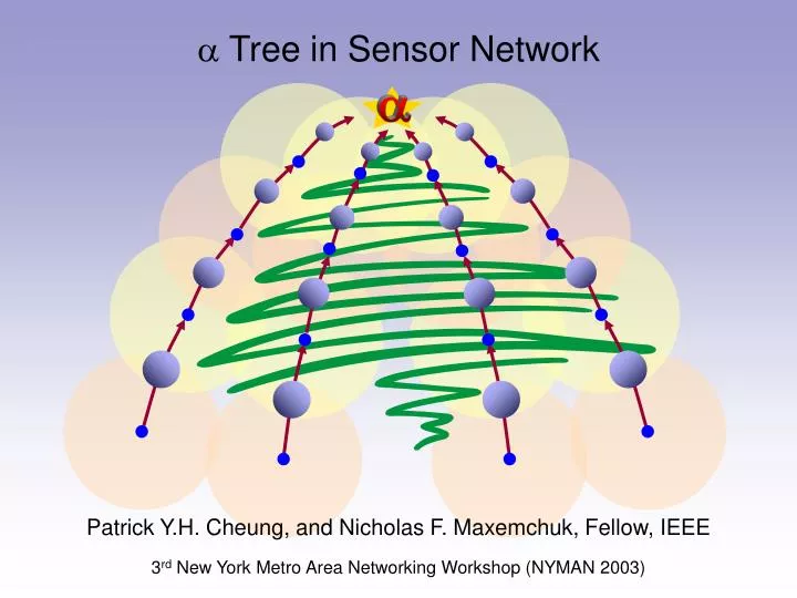
a. Tree in Sensor Network. Patrick Y.H. Cheung, and Nicholas F. Maxemchuk, Fellow, IEEE. 3 rd New York Metro Area Networking Workshop (NYMAN 2003). NYMAN 03. xxxxx xxx. Overview. Routing Problem in Sensor Network The Tree Algorithm Performance Evaluation Work in Progress. a.

E N D
a Tree in Sensor Network Patrick Y.H. Cheung, and Nicholas F. Maxemchuk, Fellow, IEEE 3rd New York Metro Area Networking Workshop (NYMAN 2003)
NYMAN 03 • xxxxx • xxx • ... Overview • Routing Problem in Sensor Network • The Tree Algorithm • Performance Evaluation • Work in Progress
a 1. Routing Problem in Sensor Network
Data Processing Center Sensor Sink Network Infrastructure Data Flow Routing Problem in Sensor Network Introduction
Perform data collection Compress data on the way Impulse arrival process triggered by an event Sensor Network Point-to-point communications Data is transparent Poisson arrival process Conventional Network Routing Problem in Sensor Network Introduction • Sensor Network vs. Conventional Network
Routing Problem in Sensor Network Introduction • If the paths are not carefully provisioned, popular routes may run out of energy before the transmission of the impulse is complete. • Two competing effects: • On one hand concentrating the data on a small number of paths increases the compression and reduces the energy. • On the other hand it increases the energy expended by those nodes and decreases the network lifetime.
Routing Problem in Sensor Network The Routing Problem • Objective: To choose paths through the sensor network to the sinks that maximize the lifetime of the network by minimizing energy consumption.
Routing Problem in Sensor Network Our Approach • Phase 1: Minimize the total energy, taking into account the amount of aggregation that can be performed along the paths. • Phase 2: Avoid overloading the popular paths by considering the energy expended by the intermediate nodes.
Routing Problem in Sensor Network Our Approach • Phase 3: Take into account congestion and energy deficits and use deflection routing to move packets in directions that are preferable based on actual network use. • The tree algorithm is a response to the challenge in Phase 1.
a 2. The Tree Algorithm
The Tree Algorithm Basic Concepts • It is the same as the Dijkstra’s Algorithm, except that we label the next closest node with (distance to the destination) • The parameter (0<<1) is adjusted according to the data aggregation performance, in order to find topologies which minimize total energy costs.
The Tree Algorithm Effects of • Consider the extreme cases: • No data reduction Optimal topology: Minimum Depth Tree (MDT) = 1 • 100% data reduction (i.e. two msgs. in, one msg. out) Optimal topology: Minimum Spanning Tree (MST) = 0 • In general, decreases as the amount of compression increases.
MDT ( = 1) MST ( = 0) Tree The Tree Algorithm Effects of • How affects the “shape” of a tree.
[5.5] [5.5] [5.5] 3 3 3 3 4 3 4 3 4 4 4 4 4 4 4 [2] [2] [2] 2 2 2 5.5 5.5 5.5 2 2 2 [0] [0] [0] 1 1 1 The Tree Algorithm A Routing Example MDT ( = 1) MST ( = 0) Tree ( = 0.5)
[5.5] 3 3 3 3 4 3 4 3 4 4 4 4 4 4 [2] [0] 2 2 2 5.5 5.5 5.5 2 2 2 [0] 1 1 1 The Tree Algorithm A Routing Example MDT ( = 1) MST ( = 0) Tree ( = 0.5) [6] [4] [5.5] [4] [5] [5.5] [5] 4 [2.5] [1] [0] [0]
[5] 3 3 4 3 4 4 4 4 [0] [1] 2 2 5.5 5.5 2 [0] [0] 1 1 The Tree Algorithm A Routing Example MDT ( = 1) MST ( = 0) Tree ( = 0.5) [6] [5.5] [0] [3] [4] [5.5] [2.5] 3 3 3 4 4 4 4 [2] 2 5.5 2 2 [0] 1
[6] [5.5] [0] [0] [2.5] 3 3 4 3 4 3 4 4 4 4 4 4 4 [2] [0] [1] 2 2 2 5.5 5.5 5.5 2 2 2 [0] [0] [0] 1 1 1 The Tree Algorithm A Routing Example MDT ( = 1) MST ( = 0) Tree ( = 0.5) [2.5] [5.5] 3 3
3 3 4 3 4 3 4 4 4 4 4 2 2 2 5.5 2 2 2 1 1 1 The Tree Algorithm A Routing Example MDT ( = 1) MST ( = 0) Tree ( = 0.5)
The Tree Algorithm Impacts • It makes a pioneer attempt on relating data aggregation performance to the generation of routing topologies which minimize the total energy cost for data funneling. • It can easily adapt to the variations in aggregation performances through the adjustment of a single parameter.
a 3. Performance Evaluation
Performance Evaluation Introduction • In order to evaluate the performance of the tree algorithm, we need a data aggregation model. • A data aggregation model describes the amount of data reduction that can be achieved in a network. • As a ground work, we begin with the simple Fixed-Ratio Data Aggregation Model.
L cL c2L ciL … 0 1 2 i Performance Analysis Introduction • In the fixed-ratio model, data is always compressed by the same ratio c at each forwarding node.
Performance Analysis Optimality of Tree for Fixed-Ratio Model • tree can always find the network topology with the minimum energy cost if we assume: (1) a fixed-ratio data aggregation model (2) link weight = (distance between two nodes)n, where n is the path loss exponent
wK wK-1 wK-2 w1 … 0 K K-1 K-2 1 Performance Analysis Optimality of Tree for Fixed-Ratio Model • Proof: Let wi = (distance between nodes i and i-1)n transmission power on the link
wK wK-1 wK-2 w1 … 0 K K-1 K-2 1 Performance Analysis Optimality of Tree for Fixed-Ratio Model By the definition of the tree algorithm, the distance from node K to node 0 DK = wK + DK-1 = wK + (wK-1 + DK-2) … = wK + wK-1 + 2 wK-2 + … + K-1 w1 ………… (1)
1 c c2 cK-1 … 0 K K-1 K-2 1 wK wK-1 wK-2 w1 Performance Analysis Optimality of Tree for Fixed-Ratio Model With a fixed compression ratio c, the total energy for sending a unit of data from node K to node 0 EK = Energy consumed on each link [wK + cwK-1 + c2 wK-2 + … + cK-1 w1] ………… (2)
Performance Analysis Optimality of Tree for Fixed-Ratio Model DK = wK + wK-1 + 2 wK-2 + … + K-1 w1 ………… (1) EK [wK + cwK-1 + c2 wK-2 + … + cK-1 w1] ………… (2) By comparing Eqns. (1) and (2), we find that DK EK if is chosen to be c. Therefore, we can prove the optimality of tree for the fixed-ratio model.
No. of bits transmitted on a link after data aggregation all links Energy Cost = (Distance)n No. of bits in a message • Define the total energy cost of a topology as Performance Analysis Simulation Results • Simulation Settings • 200 sensors are spread randomly over a 30 30 region with a sink at the center • Compression ratio = 0.8
Performance Analysis Simulation Results • The total energy costs are summarized as follows:
Performance Analysis Simulation Results Tree Topology with = 0.8 and path loss exponent = 4
a 4. Work in Progress
Work in Progress • Apply information theory to defining a generic data aggregation model, taking into consideration possible temporal and spatial correlations.
Sensing Range R Sensor Common Data among the Three Sensors Work in Progress Overlapping-Area Data Aggregation Model Larger R → Longer range of spatial correlation
Work in Progress • Based on the refined data aggregation model, evaluate the performance of tree. E.g. Percentage reduction on total energy cost with respect to node density and sensor-to-sink ratio, as compared to MST and MDT. • Investigate the relationship between the choice of and the data aggregation performances.
Work in Progress • Study the overhead in generating trees. • Find out the response of the algorithm at different levels of node mobility. • Use optimal routing to generate optimal trees and compare these trees with best trees.
References • D. Bertsekas and R. Gallager. Data Networks. Prentice-Hall, Upper Saddle River, NJ, 1992. • N.F. Maxemchuk. Video Distribution on Multicast Networks. IEEE JSAC, 15(3): 357-372, April 1997.