Download

1 / 18
190 likes | 306 Views
Neighboring Feature Clustering. Author: Z. Wang, W. Zheng, Y. Wang, J. Ford, F. Makedon, J. Pearlman Presenter: Prof. Fillia Makedon Dartmouth College. What is Neighboring Feature Clustering.

E N D
Neighboring Feature Clustering Author: Z. Wang, W. Zheng, Y. Wang, J. Ford, F. Makedon, J. Pearlman Presenter: Prof. Fillia Makedon Dartmouth College
What is Neighboring Feature Clustering • Given an m × n matrix M,where m denotes m samples and n denotes n (ordered) dimensional features, the goal is to find a intrinsic partition of the features based on their characteristics such that each cluster is a continuous piece of features. • We assume there is a natural ordering of features that has relevance to the problem being solved • E.g., in spectral datasets, such characteristics could be correlations • For example, if we decide feature 1 and 10 belong to a cluster, feature 2 to 9 should also belong to that cluster. • ZHIFENG: PLEASE IMPROVE THIS SLIDE, PROVIDE AN INTUITIVE DIAGRAM
MR spectral features and DNA Copy Number??? • MR spectral features are highly redundant suggesting that the data lie in some low-dimensional space (ZHIFENG: WHAT DO YOU MEAN BY LOW DIMENSIONAL SPACE - CLARIFY) • Neighboring spectral features of MR spectra are highly correlated • Using NFC, we can partition the features into clusters. • A cluster can be represented by a single feature, hence reducing the dimensionality. • This idea can be applied to DNA copy number analysis too. Zhifeng: Yuhang said these two are not related!! • Please explain how these are related.
Use MDL method to solve NFC • Reduce NFC into a one dimensional piece-wise linear approximation problem. • Given a sequence of n one dimensional points <x1,...,xn >, find the optimal step function-like line segments that can be fitted to the points • Fig. 1. • Piecewise linear approximation [3] [4] is usually 2D. Here we use its concept for a 1D situation. • We use minimum description length (MDL) method [2] to solve this reduced problem. • Zhifeng: define and explain MDL
Minimum Description Length (MDL) • Zhifeng, please provide a slide to define this • EXPLAIN HOW THE TRANSFORMATION IS DONE (AS IN [1]) TO GIVE 1D piece-wise linear approximation. • Represent all the points by two line segments. • Trade-off between approximation accuracy and number of line segments. • A compromise can be made using MDL. ??? • Zhifeng: it is all very cryptic, pieces of explanation are missing!
Outline • The problem • Spectral data • The abstract problem • Related work • HMM based, partial sum based, maximum likelihood based • Our approach • Problem reduced to 1D linear approximation • MDL approach
Reducing NFC to 1D Piece-Wise Linear Approximation Problem 1 • Let correlation coefficient matrix of M be denoted as C. • LetC∗ be the strictly upper triangular matrix derived from 1−|C| (entries near 0 imply high correlation between the corresponding two features). • For features from i to j (1 ≤ i ≤ j ≤ n), the submatrix C∗i:j,i:j depicts pairwise correlations. We use its entries (excluding lower and diagonal entries) as the points to be explained by a line in the 1D piece-wise linear approximation problem. • The objective is to find the optimal piece-wise line segments to fit those created points. • Points near 0 mean high correlation. We need to force high correlations among a set. Thus the points are always approximated by 0.
example • For example, suppose we have a set with points all around 0.3. • In piece-wise linear approximation, it is better to use 0.3 as the approximation. • However in NFC, we should penalize the points that stray away from 0. • So we still use 0 as the approximation. • Unlike usual 1D piece-wise linear approximation problem, the reduced problem has dynamic points (because they are created on the fly). • Zhifeng: provide figure to illustrate above example
intensit Fig. 1 high dimensional data points frequeny Fig. 2 correlation coefficient matrix Spectral data • MR spectral data • High dimensional data points • Spectral features are highly redundant (high correlation) • Find neighboring features with high correlation in a spectral dataset, such as a MR spectral dataset. Both axes are the features or the number of dimensions
Problem • Finding a low-dimensional space - • zhifeng: define low dimensional space • Curse of dimensionality • We extract an abstract problem: Neighboring Feature Clustering (NFC) • Features are ordered. Each cluster contains only neighboring features. • Find an optimal clusters according to certain criteria
Fig. 3 aCGH technology Fig. 4 aCGH data (smoothed). The X axis is log ratio Fig.5 aCGH data(segmented). The X axis is log ratio Another application (with variation) • Array Comparative Genomic Hybridization to detect copy number alterations. • aCGH data are noisy • Smoothing • Segmentation
Fig. 6 1D piece-wise approximation Related work • An algorithm trying to solve a similar problem • Baumgartner, et al, “Unsupervised feature dimension reduction for classification of MR spectra”, Magnetic Resonance Image, 22:251-256,2004 • An extensive literature on the reduced problem • The, et al, “On the detection of dominant points on digital curves”, IEEE PAMI, 11(8) 859-872, 1989 • Statistical methods…
Related work: statistical methods • HMM based • Fridlyand, et al , “Hidden Markov models approach to the analysis of array CGH data”, J. Multivariate Anal., 90, 132-153 • Partial sum based • Lipson etc., ‘”Efficient Calculation of Interval Scores for DNA copy Number Data analysis”, RECOMB 2005 • Maximum likelihood based • Picard, etc., “A statistical approach for array CGH data analysis”, BMC Bioinformatics, 6:27,2005
2. For each pair of features 1. Correlation coefficient matrix intensity frequency 3. MDL code length (revised) C1,n-1 C2,n-1 C3,n-1 4. Code length matrix … Cn-1,n C1,2 C2,3 n-1 n 1 3 2 intensity 5. Shortest path (dynamic programming) C3,n frequency C1,2 C2,n Fig. 7 our approach Framework of the method proposed
Fig. 6 1D piece-wise approximation Minimum Description Length • Information Criterion • A model selection scheme • Common information criteria are Akaike Information Criterion(AIC), Bayesian Information Criterion (BIC), and Minimum Description Length (MDL) • MDL is to encode the model and the data given the model. The balance is achieved in terms of code length
d Fig.8 encoding the data given model for each feature pair Encoding model and data given model • For each pair (n*(n-1)/2 in total) of features • Encoding model • Cluster boundary, Gaussian parameter (standard deviation) • Encoding data given model
Fig. 9 alternative representation of matrix C C1,n-1 C2,n-1 C3,n-1 … Cn-1,n C1,2 C2,3 n-1 n 1 3 2 C3,n C1,2 Fig. 10 Recursive function for the shortest path C2,n Minimize the code length • Code length matrix • Shortest path • Recursive function • Dynamic programming
Fig. 11 the revised correlation matrix and the computed code length matrix Results • We test on simulated data.