Download
1 / 40
400 likes | 523 Views
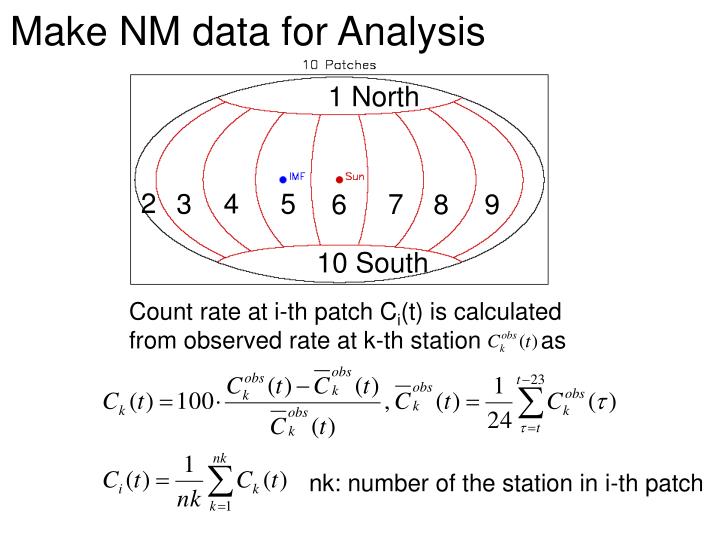
1 North. 2. 4. 3. 5. 6. 7. 8. 9. 10 South. Make NM data for Analysis. Count rate at i-th patch C i (t) is calculated from observed rate at k-th station as. nk: number of the station in i-th patch. Predict IMF from NM data. m, N: defined parameter

E N D
1 North 2 4 3 5 6 7 8 9 10 South Make NM data for Analysis Count rate at i-th patch Ci(t) is calculated from observed rate at k-th station as nk: number of the station in i-th patch
Predict IMF from NM data m, N: defined parameter An: defined from chi-square minimization • Input X: normalized NM count rate in the i-th patch Ci, i=1,10 or, deviation between i-th and j- th patch Ci,j=Ci-Cj, i,j=1,10 • Output B is compared with six types of IMF data • Bobs: Bx, By, Bz, dBx, dBy, dBz (dB(t)=B(t)-B(t-1)) by • normalized chi-square which defined as tn:number of the data in each year norm ~1: bad prediction <1: better prediction
Predicted Bz, dBz (2006) from Ci m N Number of data tn available in year 2006
Predicted (2006) from Ci,j=Ci-Cj j dBx Bx i dBy By dBz Bz m=1, N=1 m=1, N=5
Number of data tn available in year 2006 m=1, N=1 m=1, N=5
Predicted (2001) from Ci,j=Ci-Cj j i m=1, N=1 m=1, N=5
From muon data Nagoya Kuwait Hobart SaoMartinho m=1, N=5 m=1, N=1 m=1, N=5 m=1, N=1 m=1, N=5 m=1, N=1 m=1, N=5 m=1, N=1
From muon data (2006) m=1,N=1 m=1, N=1 m=1, N=1
From muon data (2006) m=1,N=5 m=1, N=5 m=1, N=5
Predicted (2006) from Ci,j=Ci-Cj j dBx Bx i dBy By dBz Bz m=1, N=1 m=1, N=5
Number of data tn available in year 2006 m=1, N=1 m=1, N=5 m=1, N=5 Num. of the gap needed to be 1/3*N
After data gap is filled j i m=1, N=5 m=1, N=5
Including CG anisotropy After correction of CG j i m=1, N=1 m=1, N=1
Including CG anisotropy After correction of CG j i m=1, N=5 m=1, N=5
For Muon data Number of data tn available in year 2006 m=1, N=1 m=1, N=5 After filling gap m=1, N=5
Correct Compton-Getting anisotropy %-deviation from 24-hour trailing average
Muon data After filling gap and correcting CG anisotropy Before j i m=1, N=5 m=1, N=5
Separate Toward and Away At time t+mΔt Bx > By → Toward Bx < By → Away
Toward m=1, N=1 m=1, N=5
Away m=1, N=1 m=1, N=5
Muon data Toward m=1, N=1 m=1, N=5
Muon data Away m=1, N=1 m=1, N=5
1 North 2 4 3 5 6 7 8 9 10 South 1 North 2 4 3 5 6 7 8 9 10 12 11 13 14 15 16 17 18 20 19 21 22 23 24 25 26 South
Toward m=1, N=1 m=1, N=5
Toward No CG correction m=1, N=1 m=1, N=1
Muon data Toward m=1, N=1 m=1, N=5
Toward Away 2006 m=1, N=1 m=1, N=1
Toward Away 2001 m=1, N=1 m=1, N=1


![Nm]](https://cdn3.slideserve.com/6300766/slide1-dt.jpg)