Download
1 / 60
600 likes | 725 Views
COLUMBIA RIVER TEMPERATURE MODEL. EPA REGION 10. Water Quality Modeling in Region 10. 3 staff in Office of Environmental Assessment Modeling to support decisions under the Clean Water Act (e.g., TMDLs, NPDES permits)

E N D
COLUMBIA RIVERTEMPERATURE MODEL EPA REGION 10
Water Quality Modeling in Region 10 • 3 staff in Office of Environmental Assessment • Modeling to support decisions under the Clean Water Act (e.g., TMDLs, NPDES permits) • Support work for R10 Offices of Water, Ecosystems and Communities, and Tribal Office
Columbia River Temperature Issue • Water temperatures exceed water quality standards to protect fish – Clean Water Act requires a restoration plan called a TMDL • States have asked EPA to take lead on TMDL • Columbia and SnakeRivers span 3 state jurisdictions • EPA has experience in this area (RBM10 model) • High profile, heavy investment project • R10’s best example of CREM guidance measures (e.g., model framework development, peer review, detailed documentation)
Two Ways to Estimate Temperatures • River Temperature Measurements (Measurement Model) • Long term scroll case readings at dams • No historic data for freely flowing river • Energy Budget (Process Model)
Concept for Measurement Model • Cross-sectionally averaged river temperatures can be estimated based upon: • Temperature Measurements at Dams (Scroll Case, Forebay, and/or Tailrace)
Concept for Process Model • Cross-sectionally averaged river temperatures can be estimated based upon: • Temperature Measurements at System Boundaries • mainstem boundaries and tributary inflows • Estimates of Surface Heat Exchange
State Estimation Approach • Treat both measurements and model estimates as random variables • Alternate approach to comparing model outputs to measurements that are assumed to be correct • Use Kalman filter algorithm to obtain “best” parameter estimates, accounting for uncertainty in both process model and measurements • Differences between observed and predicted are unbiased and uncorrelated in time
Need for Process Model • Oregon and Washington Standards for Temperature in Columbia/Snake Rivers • Allow small increases to temperature above natural conditions (e.g., 0.14 deg C in summer) • Virtually no measurements of un-impounded conditions available • Need to estimate temperatures in both impounded and un-impounded conditions
Goals of Model Development • Develop a temperature model that: • accurately simulates river temperatures • supports a TMDL analysis • Keep it non-proprietary, computationally simple and flexible • Conduct External Peer Review • 5 Reviewers (2 funded by EPA, others by industry and agencies)
System Features • Run-of-River Reservoirs • Vertical temperature stratification relatively low • Water surface elevation is relatively constant • points to potential utility of 1-D model with constant impoundment elevation • previous 1-D studies of Columbia River
MODEL SELECTION • 1-Dimensional, Time Dependent • For Impounded Condition, Estimates of Water Temperature from Process and Measurement Models Treated as Random Variables • Mixed Lagrangian-Eulerian solution technique “Reverse Particle Tracking” • reduces error due to numerical dispersion • reduces numerical instability • reduces computational burden of uncertainty evaluation
Model Name • River • Basin • Model developed in EPA Region • 10 • RBM10 is written in Fortran code and can be adapted to simulate any large scale river
TRIBUTARY INFLOW ONE-DIMENSIONAL ENERGY BUDGET MODEL SURFACE HEATTRANSFER MAIN STEM INFLOW MAIN STEM OUTFLOW
Riding the Parcel of Water Downstream - Lagrangian T2 = T1 + Net Surface Heat + Incremental Tributary Heat + Error where, T1 = initial temperature T2 = temperature after one time step
RBM10 Calculation Method • Mixed Lagrangian-Eulerian technique • “Reverse Particle Tracking” • reduces error due to numerical dispersion • reduces numerical instability • reduces computational burden of uncertainty evaluation • allows incorporation of diffusion processes
Reverse Particle Tracking 1. Compute travel time/velocities through each element 2. Track a parcel of water to its position at beginning of time step 3. Position will probably be between element boundaries 4. Estimate previous temp based on interpolation 5. Run parcel downstream, adding surface heat at each element 6. If element has a tributary, calculate flow-weighted avg temp 7. Continue adding heat and incorporating tribs 8. When time step has elapsed, stop
Elements of RBM10 Framework • Boundaries of Simulated System • System Topology • Geometry/Hydrodynamics • Boundary Inputs (Flow and Temperature) • Heat Budget Inputs based on Meteorology
Boundaries and Topology Dworshak (North Fork) Snake River segments elements Tucannon Clearwater above N.Fork Lewiston Airport Simulated Reach Snake @ Brownlee Dam Weather Station Advective Inputs (flow and temperature)
Geometry/Hydrodynamics • Mainstem Geometry for Free-Flowing Reaches • Need cross-sectional profiles of the river bottom • Open channel hydraulics relationships • HEC-RAS model • gradually varied flow is assumed • provides cross-sectional area and top width over the range of observed flows • area used to estimate velocity, width used to estimate surface area for heat exchange
Geometry/Hydrodynamics • Freely-Flowing Reaches – cont. • Leopold relationships determine width and cross sectional area for un-impounded reaches (e.g., Clearwater River) • Y = a*X^b • where, Y = cross sectional area or width • X = flow • a, b = coefficients based on regression
Geometry/Hydrodynamics • Mainstem Geometry for Impounded Reaches • Simple : constant geometry of model elements (e.g., cross-sectional area, width, volume) • Exception: Grand Coulee Dam • Storage reservoir with variable elevation • Volume-elevation relationships are used to vary geometry of model elements
Geometry/Hydrodynamics • Velocity • Continuity V = Flow / X-Area • For reservoir segments, x-area is constant • For river segments, x-area varies based on flow
Surface Heat Exchange Surface Heat Exchange = Net Absorbed Radiation - Water Dependent Exchange (J1 + J2) (J3 + J4 + J5) where, J1 = Net Solar Short Wave Radiation J2 = Net Atmospheric Long Wave Radiation J3 = Longwave Back Radiation From Water J4 = Conduction J5 = Evaporation
Meteorological Data Needed to Compute Heat Budget • Air Temperature • Dew Point • Wind Speed • Atmospheric Pressure • Cloud Cover
Available Data • On the one hand… • Long term records are available for meteorology, tributary flow, and water temperature, enabling: • long term simulations • evaluation of system variability, and • comparison of simulations to monitored temps
Data Limitations • On the other hand… • Mainstem Temperature Monitoring • Monitoring at Dams Not Designed for Assessment of River Temperature • Limited Quality Control/Quality Assurance • Tributary Temperature Monitoring • Discontinuous Record • Unknown Quality Control/Quality Assurance • Meteorology • Limited Geographical Coverage
Important Assumptions • Meteorology • Described by five regional weather stations • Mainstem Flow • Constant elevation for impounded reaches except Grand Coulee • Leopold relations developed from gradually-varied flow methods for un-impounded reaches • Tributary Temperatures • Mohseni relations developed from local air temperature and weekly/monthly river monitoring
Important Assumptions • Groundwater • Hyporheic flow does not significantly change the cross-sectionally averaged temperature in un-impounded conditions • Measurement Model • Tailrace monitoring represents best available measure of cross-sectionally averaged temperatures
PARAMETER ESTIMATION • Identify parameters that govern rates of energy transfer in the system • Some are well known (e.g., solar declination) • Some are less well known (e.g., evaporation rates) • Two parameters that are less known are to be varied • evaporation rates • assignment of area covered by 5 meteorological stations
ACCEPTANCE CRITERIA • Estimates for evaporation rates and meteorological station assignment are varied to satisfy criteria for model acceptance • Acceptance criteria (Kalman Filter characteristics): Differences between simulated and measured are unbiased and uncorrelated in time Observed variance of differences equals theoretical variance of differences
Model Evaluation Process A variety of evaluations have been conducted throughout the model development process, including: • Measurement variation evaluation (forebay, tailrace, scrollcase) • Comparison of simulated to measured (tailrace) temperatures • Comparison of un-impounded simulations with measurements from nearly un-impounded river (one dam) • Comparison: simulations vs transect measurements (special study) • Review of other temperature modeling studies in the region • Sensitivity to tributary inputs • Code tests: Eulerian vs Reverse Particle Tracking schemes
Error Estimates from Other Studies • RISLEY (1997) - Tualatin RiverMax Mean Difference = 3 Deg C Mostly < 1 Deg C • BATTELLE-MASS1 (2001) - Columbia RiverRMS Error = 0.59 - 1.52 Deg C • HDR/PORTLAND STATE/IPC (1999) - Snake RiverAME = 0.6-2.3 Deg C (1992 data) AME = 0.5-2.0 Deg C (1995 data) • CHEN (1996) - Grande Ronde RiverError = -2.20 - 8.28 Deg C (Summer Max) Error = -1.21 - 7.69 Deg C (Avg 7-day Max)