Download
1 / 33
330 likes | 440 Views
Great divide of macroeconomics. Aggregate supply and “economic growth”. Aggregate demand and business cycles. The Great Divide. Classical macro: - Full employment - Flexible wages and prices - Perfect competition and rational expectations

E N D
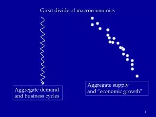
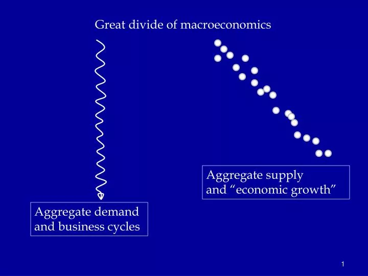
Great divide of macroeconomics Aggregate supply and “economic growth” Aggregate demand and business cycles
The Great Divide Classical macro: - Full employment - Flexible wages and prices - Perfect competition and rational expectations - Only “real” business cycles, and all unemployment is voluntary and efficient Keynesian macro: - Underutilized resources - Inflexible (or fixed) wages and prices - Imperfect competition and behavioral expectations - Yes, business cycles, with persistent slumps, involuntary unemployment, and macro waste.
Understanding business cycles Major elements of cycles • short-period (1-3 yr) erratic fluctuations in output • pro-cyclical movements of employment, profits, prices • counter-cyclical movements in unemployment • appearance of “involuntary” unemployment in recessions Historical trends • lower volatility of output, inflation over time (until 2008) • movement from stable prices to rising prices since WW II
Output gaps and business cycles Large GDP “gap”
U.S. Beveridge curve Bureau of Labor Statistics
Major approaches to business cycles • “Keynesian cross” (Econ 116): useful for intuition • AS-AD with p and Y (Econ 116): obsolete • IS-LM: for period of gold standard • IS-MP (Econ 122) • Dynamic AS-AD model: mainstream Keynesian macro • Open-economy in short run: Mundell-Fleming: Very important approach to open economy
IS-MP model The major tool for showing the impact of monetary and fiscal polices, along with the effect of various shocks, in a short-run Keynesian situation. Key assumptions • Fixed prices (P=1 and π = 0); or can have fixed inflation • Unemployed resources (Y < potential Y = Jones’s natural Y) • Closed economy (in Jones, but inessential and considered later) • Goods markets (IS) and financial markets (MP)
IS curve (expenditures) Basic idea: describes equilibrium in goods market. Finds Y where planned I = planned S or planned expenditure = planned output. Basic set of equations: • Y = C + I + G • C = a + b(Y-T) • T = T0 + τ Y [note assume income tax, τ = marginal tax rate] • I = I0 – dr [note i = r because zero inflation] • G = G0
which gives the IS curve: (IS) Y =a - bT0 + G0 + I0 - dr 1 - b(1- τ) (IS) Y = μ [A0 - dr] where A0 = autonomous spending = a - bT0 + G0 + I0 μ = simple Keynesian multiplier = 1/[(1 - b(1- τ)] which we graph as the IS curve. Note that changes in fiscal policy, investment “animal spirits,” consumption wealth effect SHIFT IS CURVE HORIZONTALLY.
IS curve r = real interest rate IS(G, T0, …) Y = real output (GDP)
IS curve r = real interest rate IS(G’, T0, …) IS(G, T0, …) Y = real output (GDP)
MP curve (monetary policy/financial markets) The simplest MP curve says that the Fed sets the short term interest rate (i). Inflation gives real interest rate. This is Chapter 12 in Jones. (MP) r = i - π
IS-MP diagram in Jones r = real interest rate E MP(π*) re IS(G, T0, …) Ye Y = real output (GDP)
Let’s go right to the real stuff • In reality, the Fed has a “dual mandate”(see below). • This is usually represented by the Taylor rule. • Let’s skip the simple case and go right there. (This is Yale.)
The Dual Mandate Fed’s dual mandate (Federal Reserve Act as amended): “promote effectively the goals of maximum employment, stable prices and moderate long-term interest rates.” In practice (FOMC statement January 2012): “The Committee judges that inflation at the rate of 2 percent, as measured by the annual change in the price index for personal consumption expenditures, is most consistent over the longer run with the Federal Reserve's statutory mandate.” “The maximum level of employment is largely determined by nonmonetary factors that affect the structure and dynamics of the labor market…In the most recent projections, FOMC participants' estimates of the longer-run normal rate of unemployment had a central tendency of 5.2 percent to 6.0 percent”
The Taylor rule 1. John Taylor suggested the following rule to implement the dual mandate: (TR) i = π + r* + b(π-π*) + cy (b, c > 0) Here r* is the equilibrium real interest rate, π inflation rate, π* is inflation target, y is % output gap [(Y-Yp)/Yp], b and c are parameters.
The Taylor rule 1. John Taylor suggested the following rule to implement the dual mandate: (TR) i = π + r* + b(π-π*) + cy Here r* is the equilibrium real interest rate, π inflation rate, π* is inflation target, y is % output gap [(Y-Yp)/Yp], b and c are parameters. 2. We will ignore inflation for now to simplify. So π = π* = 0 and we have the simplified monetary policy rule: (MP) r = r* + c[(Y- Yp) /Yp] Later on, we will introduce inflation but that doesn’t change anything important.
Taylor’s rule (IS) Y = μ [A0 - dr] (MP) r = r* + c[(Y- Yp) /Yp] And the equilibrium is: Y = μ {A0 – d[r* + c(Y- Yp)/Yp]} Y = μ {A0 – dr* –dcY + ξ} Y = μ {A0 – dr* + ξ}/(1+ μdc) Y = [μ/(1+μdc)]A0 + φ = μ* A0 + φ
Algebra of IS-MP Analysis IS-MP Equilibrium This is Main Street + Wall Street Y = μ* A0 + φ where μ* = μ/(1 + μdc) = multiplier with monetary policy. μ= simple multiplier > μ* ; A0 = autonomous spending = a - bT0 + G0 + I0 Note impacts on output: Positive: G, I0, NX, -T Negative: risk premium, inflation shock (do later)
IS-MP diagram r = real interest rate MP(r*, π, π*) E re IS(G, T0, trade…) Ye Y = real output (GDP)
1. What are the effects of fiscal policy? • A fiscal policy is change in purchases (G) or in taxes (T0,τ), holding monetary policy constant. • In normal times, because MP curve slopes upward, expenditure multiplier is reduced due to crowding out.
Fiscal policy in normal times r = real interest rate MP re IS’ IS Y = real output (GDP)
Multiplier Estimates by the CBO Congressional Budget Office, Estimated Impact of the ARRA, April 2010
US in current recession Policy has hit the “zero lower bound” four years ago.
Japan short-term interest rates, 1994-2012 Liquidity trap from 1996 to today: 15 years and counting.
Fiscal policy in liquidity trap r = real interest rate IS’ IS MP re Y = real output (GDP)
Can you see why macroeconomists emphasize the importance of fiscal policy in the current environment? “Our policy approach started with a major commitment to fiscal stimulus. Economists in recent years have become skeptical about discretionary fiscal policy and have regarded monetary policy as a better tool for short-term stabilization. Our judgment, however, was that in a liquidity trap-type scenario of zero interest rates, a dysfunctional financial system, and expectations of protracted contraction, the results of monetary policy were highly uncertain whereas fiscal policy was likely to be potent.” Lawrence Summers, July 19, 2009