Download
1 / 29
290 likes | 501 Views
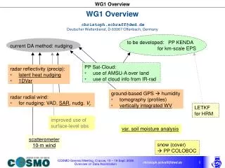
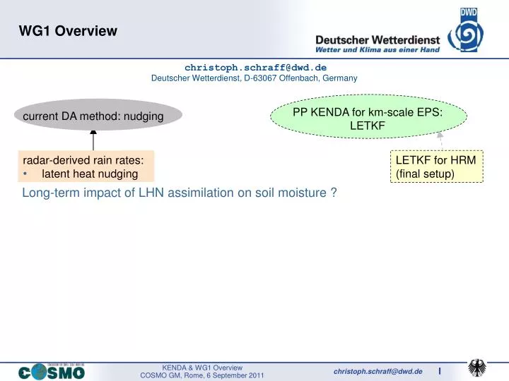
current DA method: nudging. WG1 Overview. christoph.schraff@dwd.de Deutscher Wetterdienst, D-63067 Offenbach, Germany. PP KENDA for km-scale EPS: LETKF. radar-derived rain rates: latent heat nudging. LETKF for HRM (final setup). Long-term impact of LHN assimilation on soil moisture ?.

E N D
current DA method: nudging WG1 Overview christoph.schraff@dwd.deDeutscher Wetterdienst, D-63067 Offenbach, Germany PP KENDA for km-scale EPS: LETKF radar-derived rain rates: • latent heat nudging LETKF for HRM (final setup) Long-term impact of LHN assimilation on soil moisture ?
impact of LHN on soil moisture Experiment: 18 months (April 2009 – August 2010) COSMO-DE without LHN compare with operational COSMO-DE with LHN differences in normalised soil moisture (LHN - noLHN) inside radar data domain June 2010
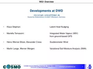
impact of LHN on soil moisture:impact on surface parameters June 2010, 12 UTC runs BIAS LHN noLHN bias reduced for different parameters
impact of LHN on soil moisture:impact on surface parameters monthly relative forecast skill (1 – rmse(LHN) / rmse(noLHN)) dew point depression 30% 35% T_2m model runs Td_2m Summer Winter Summer March 2009 Aug 2010 LHN higher soil moisture content improved T-2m , Td-2m forecasts, benefit lasts over whole forecast time
current DA method: nudging WG1 Overview christoph.schraff@dwd.deDeutscher Wetterdienst, D-63067 Offenbach, Germany PP KENDA for km-scale EPS: LETKF radar-derived rain rates: • latent heat nudging • 1DVar (comparison) LETKF for HRM (final setup) Satellite radiances: • 1DVAR: AMSU-A, SEVIRI, IASI (no benefit) • spatial AMSU-A obs errors statistics radar radial wind: • VAD (at DWD: no benefit) • nudg. Vr (being implemented) Vadim Gorin, Mikhail Tsyrulnikov: Estimation of multivariate observation-error statistics for AMSU-A data (MWR, accepted) GPS-IWV (ceased) screen-level: • scatterometer wind (OSCAT, OceanSat2) • improved T2m assimilation, adapt T_soil daytime biases in summer: • Vaisala RS-92 humidity obs dry bias bias correction operational • model warm bias (low levels) surface (snow …) PP COLOBOC
Status Overview on PP KENDA Km-scale ENsemble-based Data Assimilation christoph.schraff@dwd.deDeutscher Wetterdienst, D-63067 Offenbach, Germany Contributions / input by: Hendrik Reich, Andreas Rhodin, Roland Potthast, Uli Blahak, Klaus Stephan (DWD) Annika Schomburg (DWD / Eumetat) Yuefei Zeng, Dorit Epperlein (KIT Karlsruhe) Daniel Leuenberger, Manuel Bischof (MeteoSwiss) Mikhail Tsyrulnikov, Vadim Gorin (HMC) Lucio Torrisi (CNMCA) Amalia Iriza (NMA) • Task 1: General issues in the convective scale (e.g. non-Gaussianity) • Task 2: Technical implementation of an ensemble DA framework / LETKF • Task 3: Tackling major scientific issues, tuning, comparison with nudging • Task 4: Inclusion of additional observations in LETKF
Task 2: Technical implementation of an ensemble DA framework / LETKF analysis step (LETKF) outside COSMO code ensemble of independent COSMO runs up to next analysis time separate analysis step code, LETKF included in 3DVAR code of DWD collect obs from ]tana–3h , tana] old setup: obs from ]tana–1.5h , tana+1.5h] thinned
Task 2: Technical implementation of an ensemble DA framework / LETKF • modifications in COSMO fully implemented, but not yet in official code (also in order to have a sub-hourly update frequency) • first version LETKF (KENDA) implemented in NUMEX, to be tested still use scripts to do a few stand-alone cycles with LETKF • deterministic analysis implemented talk of Hendrik • LBC at analysis time : use (perturbed) analysis ensemble member itself instead of (temporally interpolated) LBC fields from steering ensemble system • next step: LBC from GME LETKF ensemble interpolate GME ensemble perturbations and add to deterministic COSMO-DE LBC
ensemble deterministic • deterministic run must use same set of observations as the ensemble system ! • Kalman gain / analysis increments not optimal, if deterministic background xB (strongly) deviates from ensemble mean background Analysis for a deterministic forecast run :use Kalman Gain K of analysis mean deterministic analysis recently implemented L : interpolation of analysis increments from grid of LETKF ensemble to (possibly finer) grid of deterministic run
Task 2: Technical implementation: verification for KENDA ‘stat’-utility: compute model (forecast) – obs for complete NEFF (NetCDF feedback files) : adapt verification mode of 3DVar/LETKF package need to implement COSMO observation operators with QC in 3DVar/LETKF package ( hybrid 3DVar–EnKF approaches in principle applicable to COSMO ) build COSMO modules with clean interfaces & introduce them in LETKF • no further progress • still plan to first implement upper-air obs (needed as input for VERSUS)
Task 2: Technical implementation: verification for KENDA NEFFprove (Amalia Iriza, NMA) : tool to compute and plot verification scores based on NetCDF feedback files (NEFF) • computes statistical scores for different runs (‘experiments’), focus: use exactly the same observation set in each experiment ! • select obs according to namelist values (area, quality + status of obs, … ) • compute scores (upper-air obs, screen-level obs, RR, cloud, etc.) • (for each experiment, variable, forecast time, vertical level, …) • - deterministic continuous: BIAS, RMSE, MSE • - dichotomous: accuracy, Heidke Skill Score, Hanssen and Kuiper discriminant • - ensemble scores (to be done): reliability, ROC, Brier Skill Score, • (continuous) Ranked Probability Score • plot the scores, using GNUplot (work is in progress)
Task 3: scientific issues & refinement of LETKF • lack of spread: (partly ?) due to model error and limited ensemble size which is not accounted for so far to account for it: covariance inflation, what is needed ? multiplicative (tuning, or adaptive (y – H(x) ~ R + HTPbH)) additive ((e.g. statistical 3DVAR-B), stochastic physics (Torrisi)) • localisation (multi-scale data assimilation, 2 successive LETKF steps with different obs / localisation ?) talk by Hendrik Reich • model bias • update frequency : up to now only 3-hourly • non-linear aspects, convection initiation (latent heat nudging ?) • technical aspects: efficiency, system robustness (Nov. 2012: regular ‘pre-operational’ LETKF suite)
LETKF scientific issues / refinements: investigate idealised convection • investigate LETKF in Observing System Simulation Experiments (OSSE) • apply LETKF to idealized convective weather systems, tune LETKF settings (localization, covariance inflation) • quantify + reduce spin-up time to assimilate convective storm by LETKF MeteoSwiss: plan for 2-year project not accepted • however master thesis (5 months): Manuel Bischof, MeteoSwiss perturbations of the storm environment for ensemble generation: • wind speed, temperature (low-level stability), and (low-level) humidity all suitable to perturb • meaningful perturbation amplitudes: 2 m/s, 0.25 K, 2 %
LETKF scientific issues / refinements: model error estimation • stochastic physics (Palmer et al., 2009) : by Lucio Torrisi, available Oct. 2011
LETKF scientific issues / refinements: model error estimation • objective estimation and modelling of model (tendency) errors (not to be confused with forecast errors) M. Tsyrulnikov, V. Gorin (HMC Russia) 1. set up a (revised) stochastic model (parameterisation) for model error (ME) MEM : e= *Fphys(x) + eadd • involves stochastic physics ( * Fphys(x) ) and additive components eadd andincludes multi-variate and spatio-temporal aspects • model error model parameters: (E(), D(), D(eadd)) 2. develop MEM Estimator : estimate parameters by fitting to statistics from real forecast (COSMO-RU-14) and observation (radiosonde) tendency data, using a revised (maximum likelihood based) method (tested using bootstrap) 3. develop ME Generator embedded in COSMO code 4. develop MEM Validator: exactly known ME in OSSE set-up, retrieve with MEM Estimator The reproducibility of the MEM parameters is not yet established !
Task 4: use of additional observationsTasks 4.1, 4.2: use of radar obs • radar : assimilate 3-D radial velocity and 3-D reflectivity directly Uli Blahak (DWD), Yuefei Zeng, Dorit Epperlein (KIT Karlsruhe) 1. Implement full, sophisticated observation operators (by end 2011) • compute reflectivity from model values using Mie- or Rayleigh-scattering
sub-domain 1 sub-domain 2 MPP parallelisation: beam in an azimuthal slice has to be collected on 1 PE Tasks 4.1, 4.2: use of radar obs : radar observation operator propagation of radar beam : ‘online’ depend. on refractive index, or approximate standard atmosphere averaging over beam weighting function: weighted spatial mean over measuring volumn (cross-beam vertically / horizontally)
Tasks 4.1, 4.2: use of radar obs : radar observation operator without attenuation with attenuation of radar reflectivity by atmospheric gases + hydrometeors (using the extinction coefficients)
Task 4: use of additional observationsTasks 4.1, 4.2: use of radar obs • radar : assimilate 3-D radial velocity and 3-D reflectivity directly Uli Blahak (DWD), Yuefei Zeng, Dorit Epperlein (KIT Karlsruhe) 1. implement full, sophisticated observation operators (by end 2011) 2. apply / test sufficiently accurate and efficient approximations • by looking at the simulated obs (by March 2012) • doing assimilation experiments : OSSE setup
Task 4.3: use of GNSS slant path delay • ground-based GNSS slant path delay(early 2012, N.N.) • implement non-local obs operator in parallel model environment • test and possibly compare with using GNSS data in the form of IWV or of tomographic refractivity profiles Particular issue: localisation for (vertically and horizontally) non-local obs
Task 4.4: use of cloud info • cloud information based on satellite and conventional data Annika Schomburg (DWD / Eumetsat) • derive incomplete analysis of cloud top + cloud base, using conventional obs (synop, radiosonde, ceilometer) and NWC-SAF cloud products from SEVIRI • use obs increments of cloud or cloud top / base height or derived humidity • use SEVIRI brightness temperature directly in LETKF in cloudy (+ cloud-free) conditions, in view of improving the horizontal distribution of cloud and the height of its top • compare approaches Particular issues: non-linear observation operators, non-Gaussian distribution of observation increments
Task 4.4: use of cloud info • make observations available • aggregation / interpolation to COSMO-DE / COSMO-EU grids • regular archiving: • NWC-SAF cloud products available since May 2011: (CT: cloud type, CTT: cloud top temperature, CTH: cloud top height) • BT available since June 2011: all 12 SEVIRI channels • assumption in LETKF: no bias look at systematic differences in BT / cloud products
Task 4.4: use of cloud info BT high clouds: cold bias of model-BT, (partly ?) due to known bias in RTTOV-9
Task 4.4: use of cloud info NWC-SAF SEVIRI cloud products: example cloud type CT cloud top height CTH fractional water clds high semitransparent very high clouds high clouds medium clouds low clouds very low clouds cloud-free water cloud-free land undefined COSMO: cloud water qc > 0 , or cloud ice qi > 5 .10-5 kg/kg clc = 100 % subgrid-scale clouds clc = f(RH; shallow convection; qi ,qi,sgs) < 100 %
Task 4.4: use of cloud info cloud top height CTH distribution May – July 2011 clc > 1% clc > 20% NWC-SAF CTH ‘obs’ COSMO CTH for clc > x % clc > 50% clc > 70% clc > 90%
Task 4.4: use of cloud info cloud top height CTH distribution May – July 2011 NWC-SAF CTH ‘obs’ COSMO CTH with optimal threshold: for clc > 70 % for levels above 5000 m , for clc > 40 % for levels below 5000 m
cloud cover [%] , shading: model isoline: CTH MSG Task 4.4: use of cloud info CTH COSMO 6-h forecast, for 18 May 2011, 18 UTC clc > 0.1% clc > 30% clc > 50% clc > 70% clc > 90% optimal clc height [km]
Technical implementation ofverification for KENDA thank you for your attention
0.9 Pert 1 -0.1 Pert 2 -0.1 Pert 3 -0.1 Pert 4 +( - ) +( - ) +( - ) +( - ) +( - ) +( - ) +( - ) +( - ) local transform matrix w analysis mean analysis perturbations Wa(i) analysis error covariance (computed only in ensemble space) perturbed analyses in the (k-1) -dimensional (!) sub-space S spanned by background perturbations : set up cost function J(w) in ensemble space, explicit solution for minimisation (Hunt et al., 2007) Local Ensemble Transform Kalman FilterLETKF (Hunt et al., 2007) ensemble mean forecast k perturbed forecasts ensemble mean fcst. forecast perturbations Xb flow-dep background error cov. Pb = (k – 1) Xb (Xb)T