Download
1 / 42
420 likes | 565 Views
The Structure of the Solar Atmosphere. Hugh Hudson UC Berkeley and University of Glasgow. Scope of the Hudson sessions. Basic principles, language familiarization Flares as seen in the lower solar atmosphere CMEs and space weather from a flare perspective

E N D
The Structure of the Solar Atmosphere Hugh Hudson UC Berkeley and University of Glasgow
Scope of the Hudson sessions • Basic principles, language familiarization • Flares as seen in the lower solar atmosphere • CMEs and space weather from a flare perspective • Practicum: EUV spectroscopy with EVE
Outline of presentation • General structure of solar atmosphere - Gravity, radiation, conduction, turbulence • Model atmospheres - Semi-empirical, MHD, exospheric • Plasma physics • Simple physics of a flux tube - Loop concepts • Magnetized structures
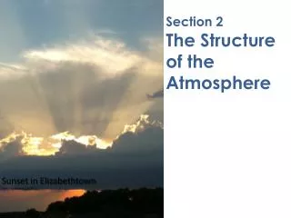
Structure of the atmosphere Wedemeyer-Bohm 2004 Corona Transition region Chromosphere Photosphere
Structure of the atmosphere Wedemeyer-Bohm 2004 Corona Transition region Chromosphere Photosphere “Interface region” (=> new IRIS spacecraft)
Structure of the atmosphere (on a roughly correct aspect ratio)
Gravity is strong • The effect of gravity can be seen via this truer scale – but still an incorrect one • Flows and other factors create the complicated structures in Wedemeyer’s cartoon • Gravity is a powerful agent; g ~ 274 m/s2 at the photosphere itself The “spicule forest” results in vertical scales much larger than the ~2,000 km of standard models
Radiation is strong • The photospheric radiation field is intense, and has dynamical consequences because of finite optical depth • Reasonably competent 1D static models (T, nvs height) can be made with gravity and radiative-transfer theory alone: the “semi-empirical models” • Such models are forced to fit the spectrum, and thus provide access to basic astrophysical knowledge such as elemental abundances • The independent parameter in a semi-empirical model is the optical depth t, normally scaled at the 5000 Å continuum
Thermal conduction is strong • Classical theory of thermal conductivity in a plasma (“Spitzer conductivity”) gives the energy flux as Fc = -k0T5/2dT/ds, suitable for fluid (MHD) descriptions; more complex transport theory involves B • In the collisionless domain, the Spitzer formula gives way to other concepts because the electron distribution function becomes non-Maxwellian • In the fluid approximation, this formula gives leads to the “RTV” and other scaling laws
Coronal loops As observed by TRACE As imagined in a cartoon What look like loops are really not stable structures Theory tends to ignore the interface region* Simple conduction theory allows the derivation of “scaling laws” *Recall
Coronal loops As observed by TRACE As imagined in a cartoon Note an oddity! What look like loops are really not stable structures Theory tends to ignore the interface region* Simple conduction theory allows the derivation of “scaling laws” *Recall
Coronal radiation(Cox & Tucker, 1969) Radiation from a complete plasma: • Optically thin • Coronal (not Saha) equilibrium • Photospheric abundances • At high temperatures, bremss • Why no Fe? Radiation from O ions only For fuller and more modern information, see CHIANTI (via SolarSoft)
Scaling laws • In conductive equilibrium, “RTV* scaling” gives T ~ (pL)1/3, where T and p are temperature and pressure at loop top • In cooling equilibrium, “Serio scaling” gives T ~ n2 as the loop depressurizes in the aftermath of an injection of energy and mass • At the base of the solar wind, the pressure depends upon the (unknown) coronal heating function. For models it is simply assumed * RTV stands for Rosner, Tucker & Vaiana (1978)
The interface region • This terminology matches the acronym of the IRIS spacecraft, the next solar observatory to be launched • The interface region separates two highly different physical domains. Generally - the sub-photosphere is a cold, (single-temperature) fluid, optically thick, collisionaly thick, and with high plasma beta - the corona is hot, optically thin, not very collisional, and with low plasma beta • We therefore expect that much of the physics that relates the corona to the interior (eg., heating) originates in this region
What is the behavior ofa coronal loop? Electrodynamic: Piddington, 1961 • Note the sub-photospheric twists, which inject currents into the atmosphere according to Ampere’s Law Hydrodynamic: Hirayama, 1974 • Note the depression of the chromosphere, the result of coronal overpressure
Loop energization P0 T0 n0 P1 > P0 T1 > T0 n1 > n0 Transition region Photosphere Footpoint in quiet field Footpoint in energized field An increase of coronal plasma temperature forces new material up from the chromosphere, increasing both pressure and density
Coronal currents and dynamic “loops” • Parallel currents in the corona (ie, J || B) result from twists present in sub-photospheric fibril fields that emerge through the surface. • At the opposite ends of a loop, a conflicting condition on the injected current must generally prevail. • No static MHD solution of this problem seems possible
A semi-empirical model • This is a standard example. Note the height and column-density scales: really the opacity t is the independent variable here • Note also the array of spectral features, including the IR and mm-wave continuum (cf. ALMA) • The photosphere (t5000A = 1) has a column density of 2-3 g/cm2 (about one Thomson length) and a density of ~1013 kg/m3 • The corona seems too low! This is because of dynamical effects Vernazza et al., 1981
What is really happening in the interface region? • Surface convection launches wave energy into it • Shock waves will form because of dispersion • Differential magnetization exists • Non-convective electric fields will occur locally • Ionization will depart from equilibrium locally • In short, kinetic physics will ultimately be needed. But, in the meanwhile, we have single-fluid MHD approaches
Interior-to-corona modeling of the interface region Perspective view (right) of the magnetic field in a small domain of an interior-to-corona MHD simulation (Abbett & Fisher, 2012). Note the magnetic complexity in the interface region
Exospheric models? • Basic plasma physics starts with particles, treated at the microscopic level kinetically • The distribution function of these particles, in general, is not Maxwellian (cf. Scudder theory of “velocity filtration”) • If the plasma has low collisionality, these complications must be dealt with (e.g., Størmer theory and adiabatic-motion theory) • Størmer* theory in the coronal context (Elliot, 1973): coronal non-thermal energy storage without twist • Do adiabatic drift motions make this idea impractical? * Next slide
Carl Størmer With Birkeland, observing the aurora (?) in 1910
Better models, still MHD • Three-dimensionality • Time dependence (hydrodynamics) • Magnetic field (MHD) • Efficient radiative transfer algorithms Rutten Hansteen Carlsson Nordlund
Better models Representative simulations • Shock waves form • Large temperature excursions result • The VAL-C model (blue line) misses in important details both in space and time • Even these “better” models omit 99% of the plasma physics, since they rely upon one-fluid MHD theory Courtesy Sven Wedemeyer-Bohm
A basic problem Why is the chromosphere so hot? Carlsson & Stein, 1995
A basic problem Why is the interface region so hot? • These simple models immediately miss the temperature minimum! • In fact, the temperature minimum should asymptotically approach the microwave background, 3 K: Carlsson & Stein, 1995
Structure of the atmosphere Wedemeyer-Bohm 2004 Photosphere Chromosphere Transition region Corona “Interface Region” (=> new IRIS spacecraft)
Coronal magnetism 1:Basic physics • Zeeman splitting allows for the remote sensing of magnetic field • The full Stokes parameters allow one to determine the line-of-sight and transverse components • This is possible in the photosphere, and maybe in the chromosphere and corona, but with caveats Hale et al. 1919
Coronal magnetism 2:HMI spectral response Tunable filter and Fe I 6173.3433 Å line Fixed filter
Coronal magnetism 3:HMI magnetograms Line-of-sight field and intensity, 2 July 2012
Recall energy storage as currents MHD version of Ampère’s Law j = B/m Twisting the field produces “free energy” in the form of its inductive field. Assume ~ steady state, with negligible gravitational forces and pressure gradients (low-beta corona). Then Force-free condition,i.e., the field and current are aligned J xB = 0 This means that curl B =a xB with the “force-free parameter” a being constant in the field direction
Coronal magnetism 5:Extrapolation techniques • Potential Field Source Surface (PFSS) assumes a = 0 (no electric currents) • Linear Force Free assumes a = constant • Nonlinear Force Free assumes a = a (x, y) • Geometricalrelies upon striations viewed in the image as a quantitative guide (Malanushenko et al. 2009)
Solar active regions • Sunspots, faculae, plage • Three-dimensionality (Wilson depression, hot-wall effect, “loops”) • p-mode absorption Scherrer et al, 2012
Conclusions • The nature of the solar atmosphere, and its physics, remain ill-understood • The “interface region” is particularly important, even though often ignored in coronal theories • We have many new tools now that will let us explore the behavior of the interface region more fully – ie, its future is bright • The MHD approximation must be viewed with great caution
Stephanie’s plasma pageshttp://sprg.ssl.berkeley.edu/~hhudson/plasma/webpage/plasma.html What do semi-empirical models, such as those of Fontenla et al (2009) suggest for plasma conditions? Note that these are (non-magnetized) fluid models, and so there is limited scope.
Stephanie’s plasma pageshttp://sprg.ssl.berkeley.edu/~hhudson/plasma/webpage/plasma.html Column density Thermal velocities Alfvén speed Plasma beta Debye parameter Gyrofrequencies Plasma Frequencies Electron collision frequency Proton collision frequency Debye length Electron inertial length Ion inertial length Electron skin depth Ion skin depth Electron mean free path Proton mean free path Hall conductivities Pedersen conductivities Cowling conductivity Tensor electrical conductivities Magnetization
Resources • M. Stix, 1989 “The Sun, an Introduction” (basic material on quiet Sun) • D. Billings, 1966 “A Guide to the Solar Corona” (background on solar corona) • A. Hundhausen, 1972, “Coronal Expansion and the Solar Wind” (basic theory of solar wind) • A.G. Emslie et al. 2012, “High-Energy Aspects of Solar Flares,” (overview of flares): SSR vol. 159 • F. Chen, 1984, “Introduction to Plasma Physics and Controlled Fusion” (plasma physics text) • H. Hudson, 2011, “Global Properties of Solar Flares,” SSR 158, 5 • Web resources - Living Reviews http://solarphysics.livingreviews.org/ - Nugget collections http://sprg.ssl.berkeley.edu/~tohban/wiki/index.php/RHESSI_Science_Nuggets et al. - Stephanie’s plasma pages http://sprg.ssl.berkeley.edu/~hhudson/plasma/webpage/plasma.html