Download

1 / 30
300 likes | 435 Views
MGMG 522 : Session #4 Choosing the Independent Variables and a Functional Form. (Ch. 6 & 7). Major Specification Problems. Problem with the selection of the independent variables. Problem with the functional form. Problem with the form of the error term.

E N D
MGMG 522 : Session #4Choosing the Independent Variablesand a Functional Form (Ch. 6 & 7)
Major Specification Problems • Problem with the selection of the independent variables. • Problem with the functional form. • Problem with the form of the error term.
Problems with the Selection of the Independent Variables • The choice of independent variables is up to the researcher to decide. • This freedom does not come without a cost. • Problems 1. Omitted variables 2. Irrelevant variables • Your underlying theory should give you some hints about what independent variables should be included in your regression model. • The statistical fit is less important than the underlying theory.
Case 1: Omitted Variables • It occurs when you don’t include important independent variables in your regression model when you should, either because you don’t think of them or you think of them but you can’t get the data. • True model: Y = 0+1X1+2X2+ε • Your model: Y = 0+1X1+ε* where, ε* = 2X2+ε • If X1 and X2 are not completely independent, ε* will not be independent of X1, a violation of the classical assumption #3 (all X’s are uncorrelated with ε).
Problems: • OLS is no longer BLUE. • Coefficient estimates are biased, . • , variances of the coefficient estimates decrease. See p. 4-8. • For a 2-independent variable model, it can be shown that, E(1) = 1+21 where 1 is from: X2 = 0+1X1+u and u is a classical error term • Coefficient estimates could be unbiased if 2 = 0 or 1 = 0. But, that is unlikely.
E(1) = 1+21 • The amount of bias = 21. • Or, the amount of bias = 2f(rx1,x2). • The direction of the bias can be determined by the signs of 2 and 1. For example, (-)(-)=(+) or (-)(+)=(-). • To correct for the omitted variables problem, • Think again about your theory. What other important variables could be missing? • If the signs of the included coefficient estimates are unexpected, you could probably tell the direction of the bias and have some clues about the missing variables.
Case 2: Irrelevant Variables • It occurs when you have some unnecessary independent variables in your regression model. • True model: Y = 0+1X1+ε • Your model: Y = 0+1X1+2X2+ε** where, ε** = ε-2X2 • The coefficient estimates will still be unbiased, but increase, lowing the reported t-values.
For the model, Y = 0+1X1+2X2. • If r12 ≠ 0, the variance will increase. • If r12 = 0 or the irrelevant variable is not in the regression model, the variance will stay the same. • Now, it seems like having extra unnecessary variables is not as serious a problem compared to the omitted variables problem. • In fact, we want neither one of these problems.
Four Criteria to Help You Choose the Independent Variables • Theory • t-Test • Adj-R2 • Bias • If all four conditions are met, that variable should be in your model. • If not, that variable doesn’t belong in your model. • If some conditions are met while some are not, use your judgment.
When you add an omitted variable, usually • Adj-R2 will rise • Coefficient estimates will change • When you add an irrelevant variable, usually • Adj-R2 will fall • Coefficient estimates will not change • t-values become less significant • Don’t rely on the Adj-R2 criterion alone, because it can be shown that Adj-R2 will rise if you include a variable with t-value > 1 but not significant. • Adj-R2 will also rise if you delete a variable with t-value < 1 from your regression model. See an example on pp. 173-176.
Three Methods to Avoid When Choosing Independent Variables • Data Mining • Stepwise Regression • Sequential Search • You should specify as few models as possible. • The more you look, the higher the chance you will find a model that has a good statistical fit with not much theoretical support. • Do not select a variable based on its t-value, because that technique creates a systematic bias. How?
Lagged Variable • Sometimes, the change in Y is not caused by the change in X from the current period, but from the other period. • The coefficient estimate of a lagged variable measures the change in Y this period as a result of a change in X in the other period.
Other Specification Criteria • Besides the four criteria outlined on p. 4-9, there are other specification criteria. • Ramsey’s Regression Specification Error Test (RESET) • Akaike’s Information Criterion (AIC) • Schwarz Criterion (SC)
Ramsey’s Regression Specification Error Test (RESET) • H0: There is no specification error. • H1: There is a specification error. • If F-value from the RESET is higher than the critical F-value, we can reject H0, meaning that there is a specification error. However, RESET doesn’t tell how to correct it. • If F-value from the RESET is lower than the critical F-value, we cannot reject H0, meaning that we probably have a correct specification. • RESET is more useful in confirming our model than telling us what’s wrong and how to correct our model.
AIC and SC • AIC and SC are used to compare two regression models. • Both AIC and SC penalize the addition of another independent variable if it doesn’t improve the overall fit significantly. • Between two regression models, the one with lower AIC and SC values is preferred.
Choosing a Functional Form • Now, you have a set of independent variables, you still need to specify a functional form. • That is, how Y is related to each X. • About the intercept term: • Do not suppress the intercept term even if the theory suggests. • Do not rely on the estimate of the intercept term for analysis or inference.
Different Functional Forms • Linear Form: Y = 0+1X1+ε • Double-Log Form: lnY = 0+1lnX1+ε • Semilog Form: lnY = 0+1X1+ε , or Y = 0+1lnX1+ε • Polynomial Form: Y = 0+1X1+2(X1)2+3(X1)3+ε • Inverse Form: Y = 0+1(1/X1)+ε • Theory usually suggests only the signs of the coefficients, not the functional form.
Linear Form • Y = 0+1X1+2X2+…+ε • The slope is constant. • But, the elasticity of Y with respect to X is not constant. • Unless the theory suggests otherwise, the linear form should be used.
Double-Log Form • lnY = 0+1lnX1+2lnX2+…+ε • This is another popular form besides the linear form. • It is also known as the “Log-linear” form. • The slope is not constant. • But, the elasticity of Y with respect to X is constant. • See p. 212 for more information.
Semilog Form • lnY = 0+1X1+2lnX2+ε , or Y = 0+1lnX1+2X2+ε • Similar to the Double-Log form, except that some variables, but not all, are in log form. • See p. 214 for more information.
Polynomial Form • Y = 0+1X1+2(X1)2+3(X1)3+ε • Appropriate for a model where changes in X cause Y to increase/decrease over some range and decrease/increase over other range. • See p. 217 for more information.
Inverse Form • Y = 0+1(1/X1)+ε • Appropriate for a model where the impact of an independent variable approaches zero as its value gets large. • See p. 219 for more information.
Selecting a Functional Form • Rely on your theory. What does your theory tell you about the relationships? • Do not compare Adj-R2 from a linear in variable model with a nonlinear in variable model. Because • Adj-R2 are not comparable when Y is transformed. Use for comparison instead. • Adj-R2 may look good inside the range of the sample, but could look bad outside the range of the sample.
Dummy Variables • Dummy Intercept takes the form: Y = 0+1X1+2D+ε • Dummy Slope takes the form: Y = 0+1X1+2X1D+ε • Both Dummy Intercept and Dummy Slope take the form: Y = 0+1X1+2X1D+3D+ε ** We will discuss the concept and use of dummy variables again in “Panel Data Regression” if we have time.
Appendix: General F-Test • Any F-test we’ve seen so far can be thought of as a special case of the general F-test. • The general F-test tests more than one coefficient at a time. • The null hypothesis for the general F-test is what we think is correct. • We usually want to “accept” H0. • This contrasts to the traditional way of hypothesis testing we’ve learned.
Steps in General F-Test • Specify the null and alternative hypotheses. • The null hypothesis will be used as a constraint to be put on the equation. • Calculate RSSs from the constraint and the unconstraint equations. • If the fits of the two equations are not significantly different, we will “accept” H0. If the fits are significantly different, reject H0.
F-statistic: • RSSC = Residual Sum of Squares from the constraint equation • RSSU = Residual Sum of Squares from the unconstraint equation • M = # of constraints • K = # of independent variables in the unconstraint equation • n = # of observations
Example of General F-Test • Y = 0+1X1+2X2+3X3+4X4+ε ----- (1) • Suppose you think 1=3=4=0 • In other words, Y = 0+2X2+ε. ----- (2) • Therefore, your H0 is 1=3=4=0. • And your H1: The original model fits the data OK. • You’ll run OLS of (1) and obtain RSSU. • You’ll run OLS of (2) and obtain RSSC. • Substitute RSSU and RSSC from (1) and (2) into the F-statistic formula. • Then, compare your F-value with the critical F-value and make the decision whether or not to reject H0. • Note for this example, K = 4, M = 3.
Chow Test • Chow test is a test whether two data sets can be combined into one data set because the slopes are not statistically different. • Put differently, there is no structural change in the model between the two data sets (e.g., before and after a war.) • H0: Slopes in the two data sets are not different (no structural change). • H1: Slopes in the two data sets are different (there is structural change).
Steps in Chow Test • Run two separate OLS regressions with the same specification for each data set and record RSS from each data set. Call these, RSS1 and RSS2. • Combined the two data sets into one and run OLS with the same specification again, and record RSS. Call it, RSST. K = # of independent variables N1 = # of observations in sample 1 N2 = # of observations in sample 2 • Reject H0 if F-value > critical F-value.