Download
1 / 15
150 likes | 604 Views
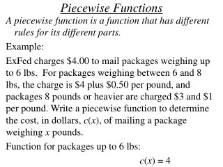
Graphing Functions - Piecewise Functions. Note: graphing piecewise functions on a calculator is not usually required by instructors. The following directions on graphing piecewise functions are mainly for the curious. Example: graph function f given by .

E N D
Graphing Functions - Piecewise Functions • Note: graphing piecewise functions on a calculator is not usually required by instructors. The following directions on graphing piecewise functions are mainly for the curious.
Example: graph function f given by ... Graphing Functions - Piecewise Functions • Graphing piecewise functions is one of the biggest challenges facing students of mathematics. These can be done on the calculator, but it does take some time to key in the expression. An example will be done now, with an explanation of the process later.
Graphing Functions - Piecewise Functions • Enter function f into Y1 using the TEST menu to enter the inequality symbols. • Y1 = (x2)(x 0) + (x + 1)(0 x)(x 3) + (6)(x 3) Slide 2
Graphing Functions - Piecewise Functions • Use a ZOOM|ZStandard window to graph the function. • To get a better graph, press WINDOW and make the following changes. Then press GRAPH. Slide 3
Graphing Functions - Piecewise Functions • The short vertical line at x = 3 does not belong to the graph. To correct this, press MODE, ... move the cursor to Dot in the fifth row and press ENTER. Press GRAPH and the result is the completed graph. Slide 4
Graphing Functions - Piecewise Functions • The graph does not show which endpoints are open and which are closed. Press TRACE and enter 3 (if not already at x = 3). • Notice that the cursor is on the line y = 6, as it should be. • Try x = 0. It appears the other closed point is on the line y = x + 1. Slide 5
It is helpful to understand the basic concept of how the calculator handles domain restrictions. Consider the function: Graphing Functions - Piecewise Functions • The rest of this module is to explain the reasoning behind the function that was typed into Y1 in the previous example. • Enter the function into Y1 ... and use a ZOOM|ZStandard window for the graph. Slide 6
Graphing Functions - Piecewise Functions • Now go back to Y1 and make the following changes: (1) Enter Y1 according to the following screen ... (2) and then select “” from the TEST menu. (3) Complete Y1 as follows and press GRAPH. Slide 7
Graphing Functions - Piecewise Functions • Only the right branch of the parabola is graphed. To see why this is so, consider (x 0) in the equation line. • A test inequality, such as (x 0) , evaluates as either 0 or 1. It is 0 when the statement is false, and 1 when the statement is true. • When x 0, (x 0) = 0. This yields (x2)(0) = 0 for the function value, and the point (x,0) is plotted on the graph. Slide 8
Graphing Functions - Piecewise Functions • Note that (x,0) is a point on the x axis and does not show up on the graph. • When x 0, (x 0) = 1. This yields (x2)(1) = x2 for the function value, which results in a point (x, x2) that is plotted on the graph. Slide 9
Graphing Functions - Piecewise Functions • Another way to see this is in a table. Go to TBLSET and make the following changes. • Now go to TABLE. • Compare the graph of function f with the table. Slide 10
Recall the function that was given at the beginning of the module. Graphing Functions - Piecewise Functions • When entering the function into Y1, the following format was used. Y1 = (x2)(x 0) + (x + 1)(0 x)(x 3) + (6)(x 3) Slide 11
Graphing Functions - Piecewise Functions • If x = -2, then Y1 takes the following form: Y1 = (x2)(x 0) + (x + 1)(0 x)(x 3) + (6)(x 3) = (-2)2 (1) + (-2 + 1) (0) (1) + (6) (0) = (-2) 2 + 0 + 0 = 4 In similar fashion, for all x 0, only the first part of the piecewise function y = x2 is nonzero. On the domain x 0, y = x2 is the only part of the function that is graphed. Slide 12
Graphing Functions - Piecewise Functions • If x = 1, then y = x + 1 is the only nonzero term: Y1 = (x2)(x 0) + (x + 1)(0 x)(x 3) + (6)(x 3) = (1)2 (0) + (1 + 1) (1) (1) + (6) (0) = 0 + 2 + 0 = 2 Thus, for all x in the domain 0 x 3, only the second part of the piecewise function y = x + 1 is nonzero, and is the only part of the function that is graphed. Slide 13