Download
1 / 23
230 likes | 374 Views
EE 4780: Introduction to Computer Vision. Linear Systems. Review: Linear Systems. We define a system as a unit that converts an input function into an output function. Independent variable. System operator. Linear Systems. Let.

E N D
EE 4780: Introduction to Computer Vision Linear Systems
Review: Linear Systems • We define a system as a unit that converts an input function into an output function. Independent variable System operator
Linear Systems • Let where fi(x) is an arbitrary input in the class of all inputs {f(x)}, and gi(x) is the corresponding output. • If Then the system H is called a linear system. • A linear system has the properties of additivity and homogeneity.
Linear Systems • The system H is called shift invariant if for allfi(x) {f(x)} and for allx0. • This means that offsetting the independent variable of the input by x0 causes the same offset in the independent variable of the output. Hence, the input-output relationship remains the same.
Linear Systems • The operator H is said to be causal, and hence the system described by H is a causal system, if there is no output before there is an input. In other words, • A linear system H is said to be stable if its response to any bounded input is bounded. That is, if where K and c are constants.
Linear Systems • A unit impulse function, denoted (a), is defined by the expression (x-a) (a) a x
Linear Systems • The response of a system to a unit impulse function is called the impulse response of the system. h(x) = H[(x)]
Linear Systems • If H is a linear shift-invariant system, then we can find its reponse to any input signal f(x) as follows: • This expression is called the convolution integral. It states that the response of a linear, fixed-parameter system is completely characterized by the convolution of the input with the system impulse response.
Linear Systems • Convolution of two functions is defined as • In the discrete case
Linear Systems • In the 2D discrete case is a linear filter.
1 1 1 -1 2 1 -1 -1 1 Convolution Example h f Rotate From C. Rasmussen, U. of Delaware
2 2 2 3 5 2 1 3 3 2 2 1 2 1 3 2 2 1 1 1 2 2 2 3 Convolution Example Step 1 -1 2 1 2 1 3 3 -1 -1 1 2 2 1 2 h 1 3 2 2 1 1 1 -1 4 2 -1 -2 1 f*h f From C. Rasmussen, U. of Delaware
2 2 2 3 2 1 3 3 2 2 1 2 1 3 2 2 1 1 1 2 2 2 3 Convolution Example Step 2 -1 2 1 2 1 3 3 -1 -1 1 2 2 1 2 h 1 3 2 2 1 1 1 5 4 -2 4 2 -2 -1 3 f*h f From C. Rasmussen, U. of Delaware
2 2 2 3 5 4 4 2 1 3 3 2 2 1 2 1 3 2 2 1 1 1 2 2 2 3 Convolution Example Step 3 -1 2 1 2 1 3 3 -1 -1 1 2 2 1 2 h 1 3 2 2 1 1 1 -2 4 3 -1 -3 3 f*h f From C. Rasmussen, U. of Delaware
2 2 2 3 5 4 4 -2 2 1 3 3 2 2 1 2 1 3 2 2 1 1 1 2 2 2 3 Convolution Example Step 4 -1 2 1 2 1 3 3 -1 -1 1 2 2 1 2 h 1 3 2 2 1 1 1 -2 6 1 -3 -3 1 f*h f From C. Rasmussen, U. of Delaware
2 2 2 3 5 4 4 -2 2 1 3 3 9 2 2 1 2 1 3 2 2 1 1 1 2 2 2 3 Convolution Example Step 5 -1 2 1 2 1 3 3 -1 -1 1 2 2 1 2 h 1 3 2 2 1 2 2 -1 4 1 -1 -2 2 f*h f From C. Rasmussen, U. of Delaware
2 2 2 3 5 4 4 -2 2 1 3 3 9 6 2 2 1 2 1 3 2 2 1 1 1 2 2 2 3 Convolution Example Step 6 -1 2 1 2 1 3 3 -1 -1 1 2 2 1 2 h 1 3 2 2 2 2 2 -2 2 3 -2 -2 1 f*h f From C. Rasmussen, U. of Delaware
Convolution Example and so on… From C. Rasmussen, U. of Delaware
Example = *
Example = *
Try MATLAB f=imread(‘saturn.tif’); figure; imshow(f); [height,width]=size(f); f2=f(1:height/2,1:width/2); figure; imshow(f2); [height2,width2=size(f2); f3=double(f2)+30*rand(height2,width2); figure;imshow(uint8(f3)); h=[1 1 1 1; 1 1 1 1; 1 1 1 1; 1 1 1 1]/16; g=conv2(f3,h); figure;imshow(uint8(g));
Gaussian Lowpass Filter = 4 = 2 From Forsyth & Ponce Original