Download
1 / 30
340 likes | 795 Views
8.5 Series Solutions Near a Regular Singular Point, Part I. We now consider the question of solving the general second order linear equation P ( x ) y'' + Q ( x ) y' + R ( x ) y = 0 (1)

E N D
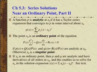
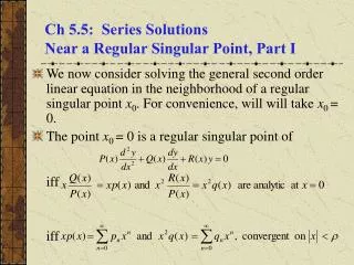
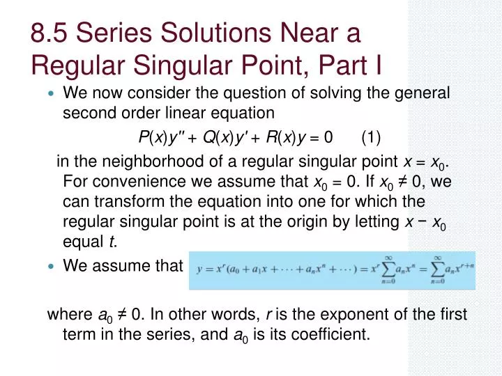
8.5 Series Solutions Near a Regular Singular Point, Part I We now consider the question of solving the general second order linear equation P(x)y'' + Q(x)y' + R(x)y = 0 (1) in the neighborhood of a regular singular point x = x0. For convenience we assume that x0 = 0. If x0 ≠ 0, we can transform the equation into one for which the regular singular point is at the origin by letting x − x0 equal t. We assume that where a0 ≠ 0. In other words, r is the exponent of the first term in the series, and a0 is its coefficient.
How to proceed As part of the solution, we have to determine: 1. The values of r for which Eq. (1) has a solution of the form (7). 2. The recurrence relation for the coefficients an. 3. The radius of convergence of the series
Example Solve the differential equation 2x2y' − xy' + (1 + x)y = 0. Answer: 1. Findthe indicial equation for diff. eq. 2. Find roots of the indicial equation called the exponents at the singularity for the regular singular point x = 0. 3. Find the general solution.
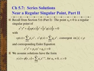
8.6 Series Solutions Near a Regular Singular Point, Part II Consider the general problem of determining a solution of the equation (1) Where (2) and both series converge in an interval |x| < ρ for some ρ > 0. The point x = 0 is a regular singular point, and the corresponding Cauchy–Euler equation (3) is
Ctd. We seek a solution of Eq. (1) for x > 0 and assume that it has the form (4) where a0 ≠ 0, and we have written y = φ(r, x) to emphasize that φ depends on r as well as x. We Get where
Indicial Equation The equation F(r ) = 0 is called the indicial equation. The roots r1 and r2 of F(r)=0 are called the exponents at the singularity; they determine the qualitative nature of the solution in the neighborhood of the singular point. Setting the coefficient of xr+nin Eq. (6) equal to zero gives the recurrence relation (8)
Unequal Roots We can always determine one solution of Eq. (1) in the form (4) We can also obtain a second solution Example
Equal Roots We can always determine one solution of Eq. (1) in the form (4) We can also obtain a second solution
Roots Differing by an Integer THEOREM 8.6.1 Consider the differential equation (1) x2y'' + x[xp(x)]y' + [x2q(x)]y = 0, where x = 0 is a regular singular point. Then xp(x) and x2q(x) are analytic at x = 0 with convergent power series expansions for |x| < ρ, where ρ > 0 is the minimum of the radii of convergence of the power series for xp(x) and x2q(x). Let r1 and r2 be the roots of the indicial equation F(r ) = r (r − 1) + p0r + q0 = 0, with r1 ≥ r2 if r1 and r2 are real.
THEOREM 8.6.1 (Ctd.) Then in either the interval −ρ < x < 0 or the interval 0 < x < ρ, there exists a solution of the form (21) where the an(r1) are given by the recurrence relation (8) with a0 = 1 and r = r1. If r1 − r2 is not zero or a positive integer, then in either the interval −ρ < x < 0 or the interval 0 < x < ρ, there exists a second solution of the form (22) The an(r2) are also determined by the recurrence relation (8) with a0 = 1 and r = r2. The power series in Eqs. (21) and (22) converge at least for |x| < ρ.
THEOREM 8.6.1 (Ctd.) If r1 = r2, then the second solution is (23) If r1 − r2 = N, a positive integer, then (24) The coefficients an(r1), bn(r1), cn(r2), and the constant a can be determined by substituting the form of the series solutions for y in Eq. (1). The constant a may turn out to be zero, in which case there is no logarithmic term in the solution (24). Each of the series in Eqs. (23) and (24) converges at least for |x| < ρ and defines a function that is analytic in some neighborhood of x = 0. In all three cases the two solutions y1(x) and y2(x) forma fundamental set of solutions of the given differential equation.
8.7 Bessel’s Equation We consider three special cases of Bessel’s equation: x2y'' + xy' + (x2 − ν2)y = 0, (1) where ν is a constant. x = 0 is a regular singular point of Eq. (1). The indicial equation is F(r ) = r(r−1)+p0r+q0=r(r−1)+r−ν2 = r2 − ν2 = 0, with the roots r = ±ν. We will consider the three cases ν = 0, ν = 1/2, and ν = 1 for the interval x > 0.
Bessel Equation of Order Zero In this case ν = 0, Eq. (1) reduces to L[ y] = x2y'' + xy' + x2y = 0, (2) and the roots of the indicial equation are equal: r1 = r2 = 0. The first solution is The function in brackets is known as the Bessel function of the first kind of order zero and is denoted by J0(x).
Bessel Equation of Order Zero The second solution of the Bessel equation of order zero is Instead of y2, the second solution is usually taken to be a certain linear combination of J0 and y2. It is known as the Bessel function of the second kind of order zero and is denoted by Y0.
General solution of the Bessel Equation of order 0 for x>0 Since The general solution of the Bessel equation of order zero for x > 0 is y = c1J0(x) + c2Y0(x).
Bessel Equation of Order One-Half Illustrates the situation in which the roots of the indicial equation differ by a positive integer but there is no logarithmic term in the second solution. Setting ν = ½ in Eq. (1) gives L[ y] = x2y'' + xy' +(x2 − ¼)y = 0. The roots of the indicial equation are r1 = ½, r2=− ½.
Bessel Equation of Order One-Half One solution of the Bessel equation of order one-half is y1 = x−1/2 sin x. The Bessel function of the first kind of order one-half, J1/2, is defined as (2/π)1/2 y1.
Bessel Equation of Order One-Half The general solution is y = c1J1/2(x) + c2J−1/2(x). where
Bessel Equation of Order One This case illustrates the situation in which the roots of the indicial equation differ by a positive integer and the second solution involves a logarithmic term. Setting ν = 1 in Eq. (1) gives L[ y] = x2y'' + xy' + (x2 − 1)y = 0.
Bessel Equation of Order One We get The general solution for x > 0 is y = c1J1(x) + c2Y1(x).
Numerical Evaluation of Bessel Functions we have shown how to obtain infinite series solutions of Bessel’s equation of orders zero, one-half, and one. In applications it is not unusual to require Bessel functions of other orders. Accurate numerical approximations can be obtained by appropriate function calls in a computer algebra system in the same way that approximations of elementary functions such as sin x and exare found.
Sections 8.2 and 8.3 Series Solutions Near an Ordinary Point, Parts I and II
Sections 8.5 and 8.6 Series Solutions Near a Regular Singular Point, Parts I and II