Download
1 / 32
330 likes | 341 Views
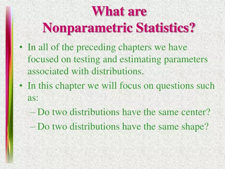
What are Nonparametric Statistics?. In all of the preceding chapters we have focused on testing and estimating parameters associated with distributions. In this chapter we will focus on questions such as: Do two distributions have the same center? Do two distributions have the same shape?.

E N D
What are Nonparametric Statistics? • In all of the preceding chapters we have focused on testing and estimating parameters associated with distributions. • In this chapter we will focus on questions such as: • Do two distributions have the same center? • Do two distributions have the same shape?
Why Use Nonparametric Statistics? • Parametric tests are based upon assumptions that may include the following: • The data have the same variance, regardless of the treatments or conditions in the experiment. • The data are normally distributed for each of the treatments or conditions in the experiment. • What happens when we are not sure that these assumptions have been satisfied?
How Do Nonparametric Tests Compare with the Usual z,t, and F Tests? • Studies have shown that when the usual assumptions are satisfied, nonparametric tests are about 95% efficient when compared to their parametric equivalents. • When normality and common variance are not satisfied, the nonparametric procedures can be much more efficientthan their parametric equivalents.
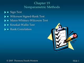
The Wilcoxon Rank Sum Test • Suppose we wish to test the hypothesis that two distributions have the same center. • We select two independent random samples from each population. Designate each of the observations from population 1 as an “A” and each of the observations from population 2 as a “B”. • If H0 is true, and the two samples have been drawn from the same population, when we rank the values in both samples from small to large, the A’s and B’s should be randomly mixed in the rankings.
What happens when H0 is true? • Suppose we had 5 measurements from population 1 and 6 measurements from population 2. • If they were drawn from the same population, the order of readings might be like this. ABABBABABBA • In this case if we summed the ranks of the A measurements and the ranks of the B measurements, the sums would be similar.
What happens if H0 is not true? • If the observations come from two different populations, perhaps with population 1 lying to the left of population 2, the observations might have the following ordering. AAABABABBB In this case the sum of the ranks of the B observations would be larger than that for the A observations.
How to Implement Wilcoxon’s Rank Test • Rank the combined sample from smallest to largest. • Let T1represent the sum of the ranks of the first sample (A’s). • Then, defined below, is the sum of the ranks that the A’s would have had if the observations were ranked from large to small.
The Wilcoxon Rank Sum Test H0: the two population distributions are the same Ha: the two populations are in some way different • The test statistic is the smaller of T1 and T1*. • Reject H0 if the test statistic is less than the critical value found in Table 7(a). • Table 7(a) is indexed by letting population 1 be the one associated with the smaller sample size n1, and population 2 as the one associated with n2, the larger sample size.
Example The wing stroke frequencies of two species of bees were recorded for a sample of n1 = 4 from species 1 and n2 = 6 from species 2. Can you conclude that the distributions of wing strokes differ for these two species? Use a = .05. If several measurements are tied, each gets the average of the ranks they would have gotten, if they were not tied! (See x = 180) H0: the two species are the same Ha: the two species are in some way different (10) (3.5) • The sample with the smaller sample size is called sample 1. • We rank the 10 observations from smallest to largest, shown in parentheses in the table. (9) (1) (8) (3.5) (7) (6) (2) (5)
(10) (3.5) (9) (1) (8) (3.5) (7) (6) (2) (5) The Bee Problem Can you conclude that the distributions of wing strokes differ for these two species? a = .05. Reject H0. There is sufficient evidence to indicate a difference in the distributions of wing stroke frequencies. • The test statistic is T = 10. • The critical value of T from Table 7(b) for a two-tailed test with a/2 = .025 is T = 12; H0 is rejected if T 12.
Large Sample Approximation:Wilcoxon Rank Sum Test When n1and n2 are large (greater than 10 is large enough), a normal approximation can be used to approximate the critical values in Table 7.
Some Notes • When should you use the Wilcoxon Rank Sum test instead of the two-sample t test for independent samples? • when the responses can only be ranked and not quantified • when the F test or the Rule of Thumb shows a problem with equality of variances • when a normality plot shows a violation of the normality assumption
The Sign Test • The sign test is a fairly simple procedure that can be used to compare two populations when the samples consist of paired observations. • It can be used • when the assumptions required for the paired-difference test of Chapter 10 are not valid or • when the responses can only be ranked as “one better than the other”, but cannot be quantified.
The Sign Test • For each pair, measure whether the first response—say, A—exceeds the second response—say, B. • The test statistic is x, the number of times that A exceeds B in the n pairs of observations. • Only pairs without ties are included in the test. • Critical values for the rejection region or exact p-values can be found using the cumulative binomial tables in Appendix I.
The Sign Test H0: the two populations are identical versus Ha: one or two-tailed alternative is equivalent to H0: p = P(A exceeds B) = .5 versus Ha: p (, <, or >) .5 Test statistic: x = number of plus signs Rejection region or p-values from Table 1.
Example Two gourmet chefs each tasted and rated eight different meals from 1 to 10. Does it appear that one of the chefs tends to give higher ratings than the other? Use a = .01. H0: the rating distributions are the same (p = .5) Ha: the ratings are different (p .5)
The Gourmet Chefs p-value =.454 is too large to reject H0. There is insufficient evidence to indicate that one chef tends to rate one meal higher than the other. H0: p = .5 Ha: p .5 with n = 7 (omit the tied pair) Test Statistic: y = number of plus signs = 2 Use Table 1 with n = 7 and p = .5. p-value = P(observe x = 2 or something equally as unlikely) = P(x 2) + P(x 5) = 2(.227) = .454
Large Sample Approximation:The Sign Test When n 25, a normal approximation can be used to approximate the critical values in Table 1.
Example You record the number of accidents per day at a large manufacturing plant for both the day and evening shifts for n = 100 days. You find that the number of accidents per day for the evening shift xE exceeded the corresponding number of accidents in the day shift xD on 63 of the 100 days. Do these results provide sufficient evidence to indicate that more accidents tend to occur on one shift than on the other? For a two tailed test, we reject H0 if |z| > 1.96 (5% level). H0 is rejected. There is evidence of a difference between the day and night shifts. H0: the distributions (# of accidents) are the same (p = .5) Ha: the distributions are different (p .5)
Which test should you use? • We compare statistical tests using Definition: Power = 1 -b = P(reject H0 when Ha is true) • The power of the test is the probability of rejecting the null hypothesis when it is false and some specified alternative is true. • The power is the probability that the test will do what it was designed to do—that is, detect a departure from the null hypothesis when a departure exists.
Which test should you use? • If all parametric assumptions have been met, the parametric test will be the most powerful. • If not, a nonparametric test may be more powerful. • If you can reject H0 with a less powerful nonparametric test, you will not have to worry about parametric assumptions. • If not, you might try • more powerful nonparametric test or • increasing the sample size to gain more power
The Wilcoxon Signed-Rank Test • The Wilcoxon Signed-Rank Test is a more powerful nonparametric procedure that can be used to compare two populations when the samples consist of paired observations. • It uses the ranks of the differences, d = x1-x2 that we used in the paired-difference test.
The Wilcoxon Signed-Rank Test • For each pair, calculate the difference d = x1- x2. Eliminate zero differences. • Rank the absolute values of the differences from 1 to n. Tied observations are assigned average of the ranks they would have gotten if not tied. • T+ = rank sum for positive differences • T- = rank sum for negative differences • If the two populations are the same, T+ and T- should be nearly equal. If either T+ or T- is unusually large, this provides evidence against the null hypothesis.
The Wilcoxon Signed-Rank Test H0: the two populations are identical versus Ha: one or two-tailed alternative Test statistic: T = smaller of T+and T- Critical values for a one or two-tailed rejection region can be found using Table 8 in Appendix I.
Example To compare the densities of cakes using mixes A and B, six pairs of pans (A and B) were baked side-by-side in six different oven locations. Is there evidence of a difference in density for the two cake mixes? H0: the density distributions are the same Ha: the density distributions are different
Cake Densities Do not reject H0. There is insufficient evidence to indicate that there is a difference in densities for the two cake mixes. Calculate: T+ = 2and T- = 5+4+3+1+6 = 19. Thetest statisticis T = 2. Rejection region:Use Table 8. For a two-tailed test with a = .05, reject H0 if T 1. Rank the 6 differences, without regard to sign.
Large Sample Approximation:The Signed-Rank Test When n 25, a normal approximation can be used to approximate the critical values in Table 8.
Summary • The nonparametric analogues of the parametric • procedures presented in Chapters 10–14 are • straightforward and fairly simple to implement. • The Wilcoxon rank sum test is the nonparametric analogue of the two-sample t test. • The sign test and the Wilcoxon signed-rank test are the nonparametric analogues of the paired-sample t test..
Key Concepts I. Nonparametric Methods 1. These methods can be used when the data cannot be measured on a quantitative scale, or when • The numerical scale of measurement is arbitrarily set by the researcher, or when • The parametric assumptions such as normality or constant variance are seriously violated. II. Wilcoxon Rank Sum Test: Independent Random Samples 1. Jointly rank the two samples: Designate the smaller sample as sample 1. Then
Key Concepts 2. Use T1 to test for population 1 to the left of population 2 Use to test for population to the right of population 2. Use the smaller of T1 and to test for a difference in the locations of the two populations. 3. Table 7 of Appendix I has critical values for the rejection of H0. 4. When the sample sizes are large, use the normal approximation:
Key Concepts III. Sign Test for a Paired Experiment 1. Find x , the number of times that observation A exceeds observation B for a given pair. 2. To test for a difference in two populations, test H0 : p= 0.5 versus a one- or two-tailed alternative. 3. Use Table 1 of Appendix I to calculate the p-value for the test. 4. When the sample sizes are large, use the normal approximation:
Key Concepts IV. Wilcoxon Signed-Rank Test: Paired Experiment 1. Calculate the differences in the paired observations. Rank the absolute values of the differences. Calculate the rank sums T- and T+ for the positive and negative differences, respectively. The test statistic T is the smaller of the two ranksums. 2. Table 8 of Appendix I has critical values for the rejection of for both one- and two-tailed tests. 3. When the sampling sizes are large, use the normal approximation: