Download
1 / 44
440 likes | 566 Views
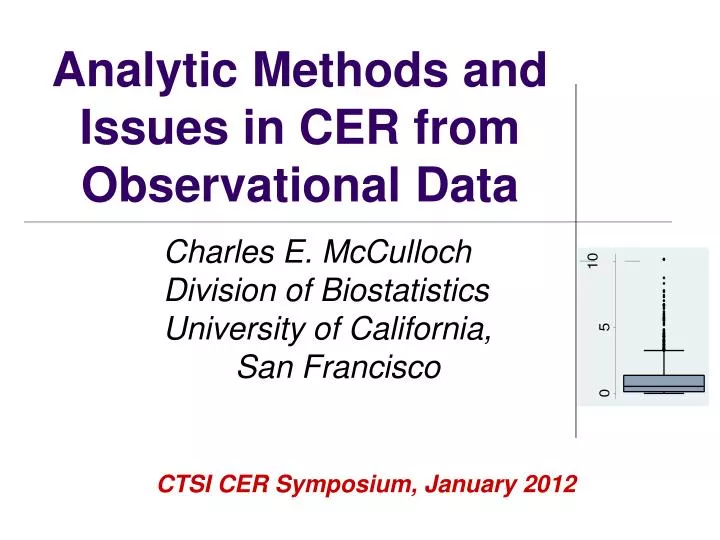
Analytic Methods and Issues in CER from Observational Data. Charles E. McCulloch Division of Biostatistics University of California, San Francisco. CTSI CER Symposium, January 2012. Outline. Some preliminary thoughts Motivating example The good old days and why they weren’t so good.

E N D
Analytic Methods and Issues in CER from Observational Data Charles E. McCulloch Division of Biostatistics University of California, San Francisco CTSI CER Symposium, January 2012
Outline • Some preliminary thoughts • Motivating example • The good old days and why they weren’t so good. • Some statistical methods • Potential outcomes and Marginal Structural Models • Propensity scores • Inverse probability weighting • Regression estimation • Instrumental variables • Some newer ideas • Recommendations
Observational CER • One of the objectives of CER is to use observational databases to answer effectiveness questions (which are invariably causal). • Basically trading what might be highly selected data that is subject to confounding for • A wealth of data available easily and cheaply, e.g., a clinical database.
To keep in mind: • “When a selection procedure is biased, taking a large sample does not help. It just repeats the basic mistake on a larger scale.” (a passage boxed for emphasis in the Stats 101 text by Freedman, et al.) • More generally: what can large samples overcome, if anything? • An under-appreciated form of selection bias in clinical databases is that the availability of data may be driven by unobserved outcomes or responses to treatment. • Put together, using a clinical database may be one of the least good ways to estimate causal effects.
Viewpoint • Both randomized and observational studies have a role in CER. • How can we be as careful as possible when analyzing and interpreting the results of observational studies and, in particular • What role can statistical analysis methods play in elucidating causal effects? • Goal: explain some of the newer approaches and why needed as well as their limitations. Focus on conceptual.
Example: treatment of depression • Does addition of an internet based cognitive behavioral component aid in treatment of depression? • Outcome = change in Beck Depression Inventory. • Control group treatment is team care approach, which has proven especially effective in the elderly. • Observational study based on clinical data. • So CER!
The good old days The issue: The treatment (the predictor of interest) is confounded by age (another predictor) since a) age is associated with the outcome (change in BDI) and b) age is associated with treatment The solution: Adjust for age in a multipredictor model
Example Treatment effect 1.4 (95% CI 0.6, 2.3)
Issues with regression adjustment Causal estimate is defined by a characteristic of the regression model. What if model is wrong (linearity/interaction)? How will we know? (Lack of overlap/extrapolation.) Lack of comparison group for older ages (plenty of controls, not many treated).
Treatment effect 3.2 (95% CI -.6, 7.1) Previously: 1.4 (95% CI 0.6, 2.3) Issues with regression adjustment (fit interaction)
Regression adjustment • To fix the issue in this linear regression situation can just center age. Use cage = age-Ave(age) = age-42.7 as a predictor instead of age in the model. • Then the treatment effect is estimated to be 1.4 (95% CI 0.5, 2.2). • But this points out the danger in using a statistical model to define the causal effect.
Another problem The old definition of confounding doesn’t really address causality. The definition is completely data-based. No information about the nature of the variables is used. What if the “other” predictor is a mediator? For example, suppose the variable we adjust for is perception of stress, instead of age. (With those having higher stress less likely to use the additional internet therapy). Then conventional wisdom is we shouldn’t adjust for it.
Message • Define your causal estimand. • Don’t let the statistical method define the target of your interest. • At the very least, be cognizant of the causal target of a statistical procedure.
Counterfactuals Imagine a hypothetical experiment in which you get to observe each participant under both the treatment and control conditions holding all else the same: Ytrt, Yctl. Like a perfect cross-over experiment. Often, we only get to observe one of Ytrt or Yctl, depending on whether the participant is in the treatment or control condition.
Counterfactuals Counter – factual Against – the truth =Lying Better? “Potential outcomes framework” or “Hypothetical outcomes framework”
Potential Outcomes – Average Causal Effect A reasonable target of inference is sometimes the average causal effect (ACE): the average of the individual causal effects across the entire population. Or perhaps the ACE in a subset of the population. E.g., the causal effect of a smoking cessation program among smokers.
Marginal structural models Consider the averages of Ytrt and Yctl across the population (Ave(Y1) and Ave(Y0)) with A=1 indicating being assigned to the treatment and 0 otherwise. A causal model: Ave(YA) = Ave(Y0) + [Ave(Y1)-Ave(Y0)]A = Ave(Y0) + [ACE]A = + A
The new order and the way forward Confounding occurs when an estimation method does not estimate the causal estimand, e.g., the average causal effect. The 800lb gorilla when trying to conduct CER from observational (especially clinical) databases is dealing with confounding. How can we estimate causal effects while doing our best to eliminate confounding?
Propensity scores: Let prop(x) be the probability of being on treatment as a function of x, the variables that determine treatment. In our example, suppose temporarily that the probability of selecting treatment only depends on age.
Propensity scores: theory Very important theoretical properties: • You only need to adjust for prop(x). • Consider individuals with the same value of prop(x). The ones receiving treatment have the same distribution of x as do those who do not. So complete overlap in the variables x is guaranteed and extrapolation is not a problem.
Propensity scores: Mean values: Ave(Trt)= 5.0, Ave(Ctl) = 4.6 (Est=0.4, p=0.57, via t-test) Within propensity score categories Prop=1/2: Ave(Trt)=4.8, Ave(Ctl)=3.3, Est=1.5 Prop=1/10: Ave(Trt)=6.8, Ave(Ctl)=6.0, Est=0.8 (Est=1.4, CI [0.4, 2.3], adj for propen) Mean values: Ave(Trt)= 5.0, Ave(Ctl) = 4.6 (Est=0.4, p=0.57, via t-test) Within propensity score categories Prop=1/2: Ave(Trt)=4.8, Ave(Ctl)=3.3, Est=1.5 Prop=1/10: Ave(Trt)=6.8, Ave(Ctl)=6.0, Est=0.8
Propensity scores: practical issues Often divide propensity scores into quintiles in order to adjust. What if not all the variables that determine treatment are measured? Or included correctly in the model? Suggests being more inclusive with both predictors and interactions. And to handle continuous predictors with flexible functional forms. So something that is easier with large databases.
Propensity scores: estimating the ACE (causal estimand) If the treatment effects vary within strata of propensity scores, then you need to weight the estimates according to the overall sample: Prop=1/2: Est = 1.5, N = 20, 64.5% of sample Prop=1/10: Est = 0.8, N = 11, 35.5% of sample Estimated ACE = 0.645*1.5 + 0.355*0.8 = 1.25 Can weight to other causal estimands.
Inverse probability weighting Instead of adjusting for the propensity score, we could use it to weight the participants. E.g., if a participant is in the treatment group and has a propensity of 1/10, then we would count that person 10 times. In that way we inflate the contribution of that participant to balance the groups. For our data: Trt estimate = 1.2 (CI -0.2, 2.5)
IPW: comments • Don’t need quintiles • Can use with longitudinal studies and time-dependent confounding. • Small probabilities (large weights) cause instability. This leads to subjective rules to deal with large weights.
Regression estimation When taking a model-based approach we could get an estimate of the causal effect for each person. Then calculate the average causal effect. This is especially useful when the regression model is not a linear regression model (e.g., a logistic model). This is because the model estimate based on the “average” subject is not the same as the average of the individual subjects’ estimates.
Regression estimation Predicted causal effect for a ctl subject Predicted causal effect for a trt subject ACE estimated to be 1.2 (CI 0.4, 2.1)
Regression estimation With sufficient data, can fit separate models for treatment and control groups. Also called G-estimation. Well known by economists as marginal estimates, built into the current version of Stata. Can get marginal estimates for subpopulations, e.g., causal effect in users of the intervention or in younger participants. But, average of conditional models may not be of scientific interest.
Doubly robust estimators There are techniques that allow you to combine the features of propensity scores or IPW estimators and regression estimation. Can, e.g., adjust for propensity score quintiles and also use regression estimation. Or use IPW and regression methods. Gives some protection against getting either the propensity scores or regression model wrong.
Instrumental variables All of the techniques described previously depend on the difficult to verify and hard to achieve assumption that all the variables needed to control for confounding have been measured and properly incorporated in the models. This is especially true once we start trying to mine clinical databases for CER purposes. The technique of instrumental variables avoids this assumption.
Instrumental variables (IVs) An instrument is a variable which: • Is a determinant of the treatment. • Is uncorrelated with any variables that jointly determine treatment and the outcome. • The entire effect of the instrument is mediated through treatment.
IVs • The classic example of an instrument is randomization to treatment, because it is 1) the primary determinant of being on treatment, 2) randomization guarantees lack of correlation with confounders, and 3) the randomization itself is often unrelated to treatment beyond assignment to treatment. • By using the instrument it is possible to get estimates of the causal effect of treatment. Angrist: “Intuitively, instrumental variables solve the omitted (confounders) problem by using only part of the variability in (treatment), specifically, a part that is uncorrelated with the omitted variables - to estimate the relationship between (treatment) and (outcome).
IVs: example of IVs Examples of instruments: • Effect of maternal smoking on birthweight, IV=state cigarette tax. • Effect of surgery on health outcomes, IV=distance to care center. • “Natural experiments”
IVs: Causal estimand • IVs do not estimate the ACE. • Instead they estimate the local average treatment effect (LATE): the average treatment effect among those who can be induced to change treatment with a change in the instrument. • For example, in the maternal smoking example, women for whom changing the tax could induce a change in smoking behavior.
IVs: Idea in linear regression Regress the treatment on the instrument, get the predicted values. This is a function of the instrument and hence represents a “portion of the treatment effect unconfounded with treatment” Regress the outcome on the predicted treatment effect to get an estimate of the causal effect.
IVs: drawbacks • The main drawback of the instrumental variables approach is the leap of faith required to believe the assumptions, which are not verifiable in practice. • If an instrumental variable is only weakly associated with treatment, then the estimate based on IVs may be quite imprecise.
Newer ideas • Not much new under the sun. • Not too surprising since many of us have been doing CER for decades. • A few new ideas, such as Propensity score calibration: Suppose you want to do a propensity score analysis but your clinical database is short on measured confounders. Build your propensity score model in a separate cohort (need not have outcomes) and figure out the degree of missclassification and its consequence on the analysis.
Recommendations • Measure confounders or consider trying instrumental variables. • Regression estimation/G-estimation is a good idea. • If using multivariate adjustment • Be liberal in including predictors, interactions and nonlinear relationships. • Center your variables. • Consider using propensity scores in strata, perhaps in addition to one of the above two methods. • Be cautious with use of IPW with small probabilities. • It’s the confounding. Doh!
We wary of methods promising easy causal estimation from observational databases • Sensitivity analyses are almost always a good idea (different methods, degree of confounding needed to overturn results).
Contact: Recommended articles: Average Causal Effects From Nonrandomized Studies: A Practical Guide and Simulated Example. JL Schafer, J Kang. Psychological Methods 2008,279–313. (somewhat technical but still readable) Instrumental Variables and the Search for Identification: From Supply and Demand to Natural Experiments. JD Angrist, AB Krueger. J Econ Perspectives, 2001, 69-85. chuck@biostat.ucsf.edu