Download
1 / 11
110 likes | 114 Views
Learn about density curves, their creation through smoothing histograms, and how they describe the overall distribution and proportion of observations within a range of values. Explore z-scores, standard normal density curves, and Chebyshev's Rule. Apply these concepts to real-world scenarios.

E N D
Interpreting Center & Variability
Density Curves • Can be created by smoothing histograms • ALWAYS on or above the horizontal axis • Has an area of exactly one underneath it • Describes the proportion of observations that fall within a range of values • Is often a description of the overall distribution • Uses μ & σ to represent the mean & standard deviation
z score Standardized score Creates the standard normal density curve Has μ = 0 & σ = 1
What do these z scores mean? -2.3 1.8 6.1 -4.3 2.3 σ below the mean 1.8 σ above the mean 6.1 σ above the mean 4.3 σ below the mean
Jonathan wants to work at Utopia Landfill. He must take a test to see if he is qualified for the job. The test has a normal distribution with μ = 45 and σ = 3.6. In order to qualify for the job, a person can not score lower than 2.5 standard deviations below the mean. Jonathan scores 35 on this test. Does he get the job? No, he scored 2.78 SD below the mean
Chebyshev’s Rule The percentage of observations that are within k standard deviations of the mean is at least where k > 1 can be used with any distribution At least what percent of observations is within 2 standard deviations of the mean for any shape distribution? 75%
Chebyshev’s Rule- what to know • Can be used with any shape distribution • Gives an “At least . . .” estimate • For 2 standard deviations – at least 75%
Normal Curve Bell-shaped, symmetrical curve Transition points between cupping upward & downward occur at μ + σ and μ – σ As the standard deviation increases, the curve flattens & spreads As the standard deviation decreases, the curve gets taller & thinner
Empirical Rule Approximately 68% of the observations are within 1σof μ Approximately 95% of the observations are within 2σof μ Approximately 99.7% of the observations are within 3σof μ Can ONLY be used with normal curves!
The height of male students at WHS is approximately normally distributed with a mean of 71 inches and standard deviation of 2.5 inches. a) What percent of the male students are shorter than 66 inches? b) Taller than 73.5 inches? c) Between 66 & 73.5 inches? About 2.5% About 16% About 81.5%
Remember the bicycle problem? Assume that the phases are independent and are normal distributions. What percent of the total setup times will be more than 44.96 minutes? First, find the mean & standard deviation for the total setup time. 2.5%