Download
1 / 21
210 likes | 320 Views
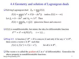
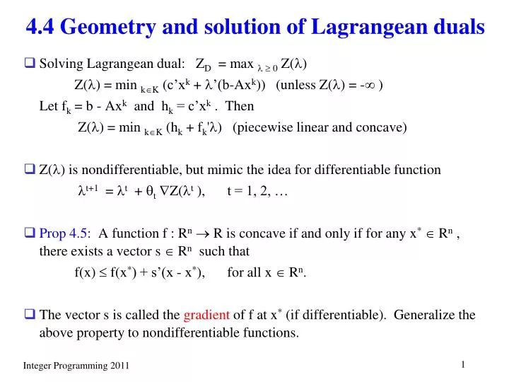
4.4 Geometry and solution of Lagrangean duals. Solving Lagrangean dual: Z D = max 0 Z() Z() = min kK ( c’x k + ’(b-Ax k )) (unless Z() = - ) Let f k = b - Ax k and h k = c’x k . Then Z() = min kK (h k + f k ') (piecewise linear and concave)

E N D
4.4 Geometry and solution of Lagrangean duals • Solving Lagrangean dual: ZD = max 0Z() Z() = min kK (c’xk + ’(b-Axk)) (unless Z() = - ) Let fk = b - Axk and hk = c’xk . Then Z() = min kK (hk + fk') (piecewise linear and concave) • Z() is nondifferentiable, but mimic the idea for differentiable function t+1 = t + t Z(t ), t = 1, 2, … • Prop 4.5: A function f : Rn R is concave if and only if for any x* Rn , there exists a vector s Rn such that f(x) f(x*) + s’(x - x*), for all x Rn. • The vector s is called the gradient of f at x* (if differentiable). Generalize the above property to nondifferentiable functions.
Def 4.3: Let f be a concave function. A vector s such that f(x) f(x*) + s’(x - x*), for all x Rn, is called a subgradient of f at x*. The set of all subgradients of f at x* is denoted as f(x*) and is called the subdifferential of f at x*. • Prop: The subdifferential f(x*) is closed and convex. Pf) f(x*) is the intersection of closed half spaces. • If f is differentiable at x*, then f(x*) = {f(x*)}. For convex functions, subgradient is defined as s which satisfies f(x) f(x*) + s’(x - x*). • Geometric intuition: Think in Rm+1 space f(x) f(x*) + s’(x – x*) s’ x* – f(x*) s’x - f(x) ( s, -1)’(x*, f(x*)) ( s, -1)’( x, f(x)) ( s, -1)’{ (x, f(x)) - (x*, f(x*)) } 0
Picture: ( s, -1)’{ (x, f(x)) - (x*, f(x*)) } 0 f(x) = f(x*) + s’(x – x*) (x, f(x)) – (x*, f(x*)) f(x) (x, f(x)) (x*, f(x*)) s (s, -1) -1 x x x*
For convex functions: ( s, -1)’{ (x, f(x)) - (x*, f(x*)) } 0 f(x) = f(x*) + s’(x – x*) f(x) (x, f(x)) – (x*, f(x*)) (x*, f(x*)) s (x, f(x)) (s, -1) -1 x x x*
Prop 4.6: Let f : Rn R be a concave function. A vector x* maximizes f over Rn if and only if 0 f(x*). Pf) A vector x* maximizes f over Rn if and only if f(x) f(x*) = f(x*) + 0’(x - x*), for all x Rn , which is equivalent to 0 f(x*). • Prop 4.7: Let Z() = min kK (hk + fk') E() = { k K: Z() = hk + fk'}. Then, for every * 0 the following relations hold: (a) For every k E(*), fk' is a subgradient of the function Z() at *. (b) Z(*) = conv( {fk : k E(*)} ), i.e., a vector s is a subgradient of the function Z() at * if and only if s is a convex combination of the vectors fk , k E(*).
Pf) (a) By definition of Z() we have for every k E(*) Z() hk + fk' = hk + fk'* + fk'( - *) = Z(*) + fk‘( - *). (b) We have shown that {fk : k E(*)} Z(*) and since a convex combination of two subgradients is also a subgradients , it follows that conv( {fk : k E(*)} ) Z(*). Assume that there is s Z(*), such that s conv( {fk : k E(*)} ) and derive a contradiction. By the separating hyperplane theorem, there exists a vector d and a scalar , such that d’fk , for all k E(*) (4.29) d’s < Since Z(*) < hi + fi'*, for all i E(*), then for sufficiently small > 0, we have, Z(* + d) = hk + fk'(* + d), for some k E(*) Since Z(*) = hk + fk'* , we obtain that Z(* + d) - Z(*) = fk’d, for some k E(*)
(continued) From (4.29), we have Z(* + d) - Z(*) . (4.30) Since s Z(*), we have Z(* + d) Z(*) + s’d. (def’n of subgradient) From (4.29), we have Z(* + d) - Z(*) < , ( d’s < ) contradicting (4.30).
Subgradient algorithm • For differentiable functions, the direction f(x) is the direction of steepest ascent of f at x. But, for nondifferentiable functions, the direction of subgradient may not be an ascent direction. However, moving along the direction of a subgradient, we can move closer to the minimum point.
Ex: f(x1, x2) = min { -x1, x1 – 2x2, x1 + 2x2 } : concave function direction of subgradient may not be an ascent direction for f, but we can move closer to the maximum point. x2 f(x) = -2 s2 = (1, 2) s1(x-x*)=0 f(x) = -1 x1 f(x) = 0 x* = (-2, 0) s2(x-x*)=0 s1 = (1, -2)
The subgradient optimization algorithm Input: A nondifferentiable concave function Z(). Output: A maximizer of Z() subject to 0. Algorithm: • Choose a starting point 1 0; let t = 1. • Given t , check whether 0 Z(t). If so, then t is optimal and the algorithm terminates. Else, choose a subgradient st of the function Z(t). (fk b-Axk ) • Let jt+1 = max {jt + t sjt , 0} (projection), where t is a positive step size parameter. Increment t and go to Step 2.
Choosing the step lengths: • Thm : (a) If t=1 t , and limt t = 0, then Z(t) ZD the optimal value of Z(). (b) If t = 0 t , t = 1, 2, …, for some parameter 0 < < 1, then Z(t) ZD if 0 and are sufficiently large. (c) If t = f [ZD* – Z(t) ] / || st ||2 , where 0 < f < 2, and ZD* ZD , then Z(t) ZD*, or the algorithm finds t with ZD* Z(t) ZD , for some finite t. • (a) guarantees convergence, but slow (e.g., t = 1/t ) (b) In practice, may use halving the value of t after iterations (c) ZD* typically unknown, may use a good primal upper bound in place of ZD*. If not converge, decrease ZD*. • In practice, 0 Z(t) is rarely met. Usually, only find approximate optimal solution fast and resort to B-and-B. Convergence is not monotone. If ZD = ZLP , solving LP relaxation may give better results (monotone convergence).
Ex: Traveling salesman problem: For TSP, we dualize degree constraints for nodes except node 1. Z() = min eE ( ce – i – j ) xe + 2 i V\{1}i ( = min eE ce xe + i V\{1}i(2 - e (i) xe ) ) e (1)xe = 2, eE(S) xe |S| - 1, S V\{1}, S , V\{1}, eE(V\{1}) xe = |V| - 2, xe { 0, 1 }. step direction is it+1 = it + t ( 2 - e (i) xe(t) ) step size using rule (c) is t = f [ZD* – Z(t) ] / i V ( 2 - e (i) xe(t) )2 (t = f [ZD* – Z(t) ] / || b-Ax(t) ||2 ) • Note that i-th coordinate of subgradient direction is two minus the number of edges incident to node i in the optimal one-tree. We do not have 0 here since the dualized constraints are equalities.
Lagrangean heuristic and variable fixing: • The solution obtained from solving the Lagrangian relaxation may not be feasible to IP, but it can be close to a feasible solution to IP. Obtain a feasible solution to IP using heuristic procedures. Then we may obtain a good upper bound on optimal value. Also called ‘primal heuristic’ • May fix values of some variables using information from Lagrangian relaxation (refer to W,177-178).
Choosing a Lagrangean dual: How to determine the constraints to relax? • Strength of the Lagrangean dual bound • Ease of solution of Z() • Ease of solution of Lagrangean dual problem ZD = max 0Z() • Ex: Generalized Assignment Problem (max problem)(refer to W p. 179): z = max j = 1n i = 1m cijxij j = 1n xij 1 for i = 1, … , m i = 1m aij xij bj for j = 1, … , n x Bmn
Dualize both sets of constraints: Z1D = minu 0, v 0 Z1(u, v), where Z1(u, v) = max j = 1n i = 1m (cij – ui – aijvj )xij + i = 1m ui + j = 1n vjbj x Bmn • Dualize first set of assignment constraints: Z2D = minu 0 Z2(u), where Z2(u) = max j = 1n i = 1m (cij – ui )xij + i = 1m ui i = 1m aij xij bj for j = 1, … , n x Bmn • Dualize the knapsack constraints: Z3D = minv 0 Z3(v), where Z3(v) = max j = 1n i = 1m (cij – aij vj )xij + j = 1n vjbj j = 1n xij 1 for i = 1, … , m x Bmn
Z1D = Z3D = ZLP For each i, conv{ x: j = 1n xij 1, xij {0, 1} for j = 1, … , n } = conv{ x: j = 1n xij 1, 0 xij 1 for j = 1, … , n } Z1(u, v), Z3(v) can be solved by inspection. Calculating Z3D look easier than calculating Z1D since there are m dual variables compared to m+n for Z1D. • Z2D ZLP • To find Z2(u), we need to solve n 0-1 knapsack problems. Also note that the information that we may obtain while solving the knapsack cannot be stored and used for subsequent optimization.
May solve the Lagrangean dual by constraint generation (NW p411-412): • Recall that ZD = maximize y subject to y + ’(Axk - b) c’xk , kK ’Awj c’wj , jJ 0 • Given (y*, *), with * 0, calculate Z(*) = min x conv(F) (c’x + *’(b-Ax)) (min (c’-*’A)x + ’b) If y*Z(*), stop y* = Z(*), = * is an optimal solution If y*>Z(*), an inequality is violated • Z(*) , ray wj s.t. (c’-*’A)wj < 0, hence ’Awj c’wj is violated • Z(*) < , extreme point xk s.t. Z(*) = c’xk + *’(b-Axk). Since y*>Z(*), y + ’(Axk - b) c’xk is violated. • Note that max/min is interchanged in NW.
Nonlinear Optimization Problems • Geometric understanding of the strength of the bounds provided by the Lagrangean dual • Let be continuous functions. Let . minimize subject to (4.31) . Let be the optimal cost. Consider Lagrangean function . • For all , and is a concave function. Lagrangean dual: . • Let . Problem (4.31) can be restated as minimize subject to .
Figure 4.7: The geometric interpretation of the Lagrangean dual
Given that , we have for a fixed and for all that , . Geometrically, this means that the hyperplane lies below the set Y. For , we obtain , that is is the intercept of the hyperplane with the vertical axis. To maximize , this corresponds to finding a hyperplane, which lies below the set Y, such that the intercept of the hyperplane with the vertical axis is the largest. • Thm 4.10: The value of the Lagrangean dual is equal to the value of the following optimization problem: minimize subject to .
Ex 4.7: Ex 4.3 revisited and , {(1, 0), (2,0), (1, 1), (2, 1), (0, 2), (1, 2), (2, 2), (1, 3), (2, 3)} {(3, -2), (6, -3), (2, -1), (5, -2), (-2, 1), (1, 0), (4, -1), (0, 1), (3, 0)} duality gap