Download
1 / 36
360 likes | 457 Views
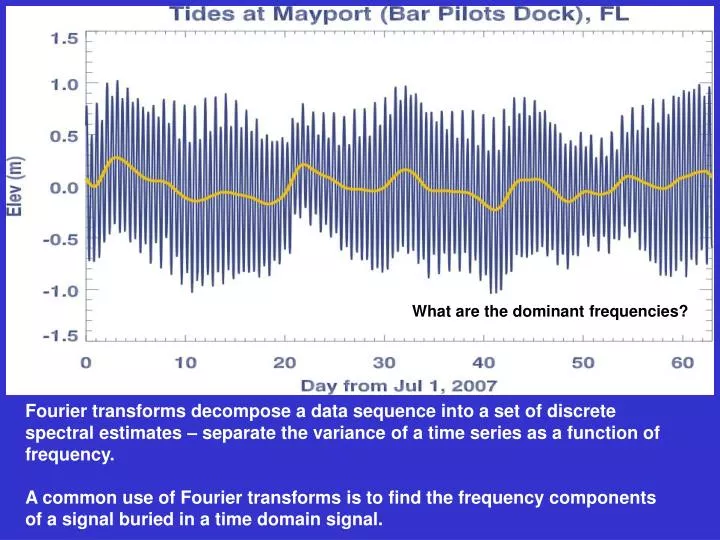
What are the dominant frequencies?. Fourier transforms decompose a data sequence into a set of discrete spectral estimates – separate the variance of a time series as a function of frequency.

E N D
What are the dominant frequencies? Fourier transforms decompose a data sequence into a set of discrete spectral estimates – separate the variance of a time series as a function of frequency. A common use of Fourier transforms is to find the frequency components of a signal buried in a time domain signal.
FAST FOURIER TRANSFORM (FFT) In practice, if the time series f(t) is not a power of 2, it should be padded with zeros
What is the statistical significance of the peaks? Each spectral estimate has a confidence limit defined by a chi-squared distribution
Spectral Analysis Approach 1. Remove mean and trend of time series 2. Pad series with zeroes to a power of 2 3. To reduce end effect (Gibbs’ phenomenon) use a window (Hanning, Hamming, Kaiser) to taper the series 4. Compute the Fourier transform of the series, multiplied times the window 5. Rescale Fourier transform by multiplying times 8/3 for the Hanning Window 6. Compute band-averages or block-segmented averages 7. Incorporate confidence intervals to spectral estimates
1. Remove mean and trend of time series (N = 1512) 2. Pad series with zeroes to a power of 2 (N = 2048) m Sea level at Mayport, FL July 1, 2007 (day “0” in the abscissa) to September 1, 2007 Raw data and Low-pass filtered data m High-pass filtered data
Spectrum of raw data m2/cpd Spectrum of high-pass filtered data m2/cpd Cycles per day
Hanning Window Hamming Window Value of the Window 3. To reduce end effect (Gibbs’ phenomenon) use a window (Hanning, Hamming, Kaiser) to taper the series Day from July 1, 2007
Hanning Window Hamming Window Kaiser-Bessel, α = 2 Kaiser-Bessel, α = 3 Value of the Window Day from July 1, 2007 3. To reduce end effect (Gibbs’ phenomenon) use a window (Hanning, Hamming, Kaiser) to taper the series
4. Compute the Fourier transform of the series, multiplied times the window Raw series x Hanning Window (one to one) m Raw series x Hamming Window (one to one) m To reduce side-lobe effects Day from July 1, 2007
4. Compute the Fourier transform of the series, multiplied times the window High-pass series x Hanning Window (one to one) m High pass series x Hamming Window (one to one) m To reduce side-lobe effects Day from July 1, 2007
High pass series x Kaiser-Bessel Window α=3 (one to one) m Day from July 1, 2007 4. Compute the Fourier transform of the series, multiplied times the window
Windows reduce noise produced by side-lobe effects Noise reduction is effected at different frequencies with Hanning window m2/cpd Original from Raw Data with Hamming window m2/cpd Cycles per day
with Hanning window m2/cpd with Hamming and Kaiser- Bessel (α=3) windows m2/cpd Cycles per day
5. Rescale Fourier transform by multiplying: times 8/3 for the Hanning Window times 2.5164 for the Hamming Window times ~8/3 for the Kaiser-Bessel (Depending on alpha)
6. Compute band-averages or block-segmented averages 7. Incorporate confidence intervals to spectral estimates Upper limit: Lower limit: 1-alpha is the confidence (or probability) nu are the degrees of freedom gamma is the ordinate reference value
0.995 0.990 0.975 0.950 0.900 0.750 0.500 0.250 0.100 0.050 0.025 0.010 0.005 7.88 6.63 5.02 3.84 2.71 1.32 0.45 0.10 0.02 0.00 0.00 0.00 0.00 10.60 9.21 7.38 5.99 4.61 2.77 1.39 0.58 0.21 0.10 0.05 0.02 0.01 12.84 11.34 9.35 7.81 6.25 4.11 2.37 1.21 0.58 0.35 0.22 0.11 0.07 14.86 13.28 11.14 9.49 7.78 5.39 3.36 1.92 1.06 0.71 0.48 0.30 0.21 16.75 15.09 12.83 11.07 9.24 6.63 4.35 2.67 1.61 1.15 0.83 0.55 0.41 18.55 16.81 14.45 12.59 10.64 7.84 5.35 3.45 2.20 1.64 1.24 0.87 0.68 20.28 18.48 16.01 14.07 12.02 9.04 6.35 4.25 2.83 2.17 1.69 1.24 0.99 21.95 20.09 17.53 15.51 13.36 10.22 7.34 5.07 3.49 2.73 2.18 1.65 1.34 23.59 21.67 19.02 16.92 14.68 11.39 8.34 5.90 4.17 3.33 2.70 2.09 1.73 25.19 23.21 20.48 18.31 15.99 12.55 9.34 6.74 4.87 3.94 3.25 2.56 2.16 26.76 24.72 21.92 19.68 17.28 13.70 10.34 7.58 5.58 4.57 3.82 3.05 2.60 28.30 26.22 23.34 21.03 18.55 14.85 11.34 8.44 6.30 5.23 4.40 3.57 3.07 29.82 27.69 24.74 22.36 19.81 15.98 12.34 9.30 7.04 5.89 5.01 4.11 3.57 31.32 29.14 26.12 23.68 21.06 17.12 13.34 10.17 7.79 6.57 5.63 4.66 4.07 32.80 30.58 27.49 25.00 22.31 18.25 14.34 11.04 8.55 7.26 6.26 5.23 4.60 34.27 32.00 28.85 26.30 23.54 19.37 15.34 11.91 9.31 7.96 6.91 5.81 5.14 35.72 33.41 30.19 27.59 24.77 20.49 16.34 12.79 10.09 8.67 7.56 6.41 5.70 37.16 34.81 31.53 28.87 25.99 21.60 17.34 13.68 10.86 9.39 8.23 7.01 6.26 38.58 36.19 32.85 30.14 27.20 22.72 18.34 14.56 11.65 10.12 8.91 7.63 6.84 40.00 37.57 34.17 31.41 28.41 23.83 19.34 15.45 12.44 10.85 9.59 8.26 7.43 41.40 38.93 35.48 32.67 29.62 24.93 20.34 16.34 13.24 11.59 10.28 8.90 8.03 42.80 40.29 36.78 33.92 30.81 26.04 21.34 17.24 14.04 12.34 10.98 9.54 8.64 44.18 41.64 38.08 35.17 32.01 27.14 22.34 18.14 14.85 13.09 11.69 10.20 9.26 45.56 42.98 39.36 36.42 33.20 28.24 23.34 19.04 15.66 13.85 12.40 10.86 9.89 46.93 44.31 40.65 37.65 34.38 29.34 24.34 19.94 16.47 14.61 13.12 11.52 10.52 48.29 45.64 41.92 38.89 35.56 30.43 25.34 20.84 17.29 15.38 13.84 12.20 11.16 49.64 46.96 43.19 40.11 36.74 31.53 26.34 21.75 18.11 16.15 14.57 12.88 11.81 50.99 48.28 44.46 41.34 37.92 32.62 27.34 22.66 18.94 16.93 15.31 13.56 12.46 52.34 49.59 45.72 42.56 39.09 33.71 28.34 23.57 19.77 17.71 16.05 14.26 13.12 53.67 50.89 46.98 43.77 40.26 34.80 29.34 24.48 20.60 18.49 16.79 14.95 13.79 55.00 52.19 48.23 44.99 41.42 35.89 30.34 25.39 21.43 19.28 17.54 15.66 14.46 56.33 53.49 49.48 46.19 42.58 36.97 31.34 26.30 22.27 20.07 18.29 16.36 15.13 57.65 54.78 50.73 47.40 43.75 38.06 32.34 27.22 23.11 20.87 19.05 17.07 15.82 58.96 56.06 51.97 48.60 44.90 39.14 33.34 28.14 23.95 21.66 19.81 17.79 16.50 60.27 57.34 53.20 49.80 46.06 40.22 34.34 29.05 24.80 22.47 20.57 18.51 17.19 Probability 1 2 3 4 5 6 7 8 9 10 11 12 13 14 15 16 17 18 19 20 21 22 23 24 25 26 27 28 29 30 31 32 33 34 35 Degrees of freedom
N=1512 Includes low frequency
N=1512 Excludes low frequency
Least Squares Fit to Main Harmonics The observed flow u’ may be represented as the sum of M harmonics: u’ = u0 + ΣjM=1Aj sin (j t + j) For M = 1 harmonic (e.g. a diurnal or semidiurnal constituent): u’ = u0+ A1 sin (1t + 1) With the trigonometric identity: sin (A + B) = cosBsinA + cosAsinB u’ = u0 + a1 sin (1t ) + b1 cos (1t ) taking: a1= A1 cos 1 b1= A1 sin 1
Using u’ = u0 + a1 sin (1t ) + b1 cos (1t ) Then: 2 = ΣN {u 2 - 2uu0 - 2ua1 sin (1t ) - 2ub1 cos (1t ) + u02 + 2u0a1 sin (1t ) + 2u0b1 cos (1t ) + 2a1 b1 sin (1t ) cos (1t ) + a12sin2 (1t ) + b12cos2 (1t ) } The squared errors between the observed current u and the harmonic representation may be expressed as 2 : 2 = ΣN [u - u’ ]2 = u 2 - 2uu’ + u’ 2 Then, to find the minimum distance between observed and theoretical values we need to minimize 2 with respect to u0 a1and b1, i.e., δ 2/ δu0 , δ 2/ δa1 , δ 2/ δb1 : δ2/ δu0 = ΣN {-2u +2u0 + 2a1 sin (1t ) + 2b1 cos (1t ) } = 0 δ2/ δa1 = ΣN { -2u sin (1t ) +2u0 sin (1t ) + 2b1 sin (1t ) cos (1t ) + 2a1 sin2(1t ) } = 0 δ2/ δb1 = ΣN {-2u cos (1t ) +2u0 cos (1t ) + 2a1 sin (1t ) cos (1t ) + 2b1 cos2(1t ) } = 0
ΣN { u = u0 + a1 sin (1t ) + b1 cos (1t ) } ΣN { u sin (1t ) = u0 sin (1t ) + b1 sin (1t ) cos (1t ) + a1 sin2(1t ) } ΣN { u cos (1t ) = u0 cos (1t ) + a1 sin (1t ) cos (1t ) + b1 cos2(1t ) } ΣN u N ΣN sin (1t ) ΣN cos (1t ) u0 ΣN {-2u +2u0 + 2a1 sin (1t ) + 2b1 cos (1t ) } = 0 ΣN u sin (1t ) = ΣN sin (1t ) ΣN sin2(1t ) ΣN sin (1t ) cos (1t ) a1 ΣN u cos (1t ) ΣN cos (1t ) ΣN sin (1t ) cos (1t ) ΣN cos2(1t ) b1 ΣN {-2u sin (1t ) +2u0 sin (1t ) + 2b1 sin (1t ) cos (1t ) + 2a1 sin2(1t ) } = 0 ΣN { -2u cos (1t ) +2u0 cos (1t ) + 2a1 sin (1t ) cos (1t ) + 2b1 cos2(1t ) } = 0 X = A-1 B Rearranging: And in matrix form: B = A X
Finally... The residual or mean is u0 The phase of constituent 1 is: 1 = atan( b1 / a1 ) The amplitude of constituent 1 is: A1 = ( b12+ a12 )½ Pay attention to the arc tangent function used. For example, in IDL you should use atan (b1,a1) and in MATLAB, you should use atan2
Matrix A is then: N ΣN sin (1t ) ΣN cos (1t ) ΣN sin (2t ) ΣN cos (2t ) ΣN sin (1t ) ΣN sin2(1t ) ΣN sin (1t ) cos (1t ) ΣN sin (1t ) sin (2t ) ΣN sin (1t ) cos (2t ) ΣN cos (1t ) ΣN sin (1t ) cos (1t ) ΣN cos2(1t ) ΣN cos (1t ) sin (2t ) ΣN cos (1t ) cos (2t ) ΣN sin (2t ) ΣN sin (1t ) sin (2t ) ΣN cos (1t ) sin (2t ) ΣN sin2(2t ) ΣN sin (2t ) cos (2t ) ΣN cos (2t ) ΣN sin (1t ) cos (2t ) ΣN cos (1t ) cos (2t ) ΣN sin (2t ) cos (2t ) ΣN cos2 (2t ) Remember that: X = A-1 B and B = u0 a1 b1 a2 b2 ΣN u ΣN u sin (1t ) X = ΣN u cos (1t ) ΣN u sin (2t ) ΣN u cos (2t ) For M = 2 harmonics (e.g. diurnal and semidiurnal constituents): u’ = u0+ A1 sin (1t + 1) + A2 sin (2t + 2)
Goodness of Fit: Σ [< uobs > - upred] 2 ------------------------------------- Σ [<uobs > - uobs] 2 Root mean square error: [1/N Σ (uobs - upred) 2] ½
Fit with M2, S2, K1
Fit with M2, S2, K1, M4, M6
Tidal Ellipse Parameters amplitude of the counter-clockwise rotary component phase of the clockwise rotary component phase of the counter-clockwise rotary component Ellipse Coordinates: ua, va, up, vpare the amplitudes and phases of the east-west and north-south components of velocity amplitude of the clockwise rotary component The characteristics of the tidal ellipses are: Major axis = M = Qcc + Qc minor axis = m = Qac - Qc ellipticity = m / M Phase = -0.5 (thetacc - thetac) Orientation = 0.5 (thetacc + thetac)
M2 S2 K1