Download
1 / 25
250 likes | 372 Views
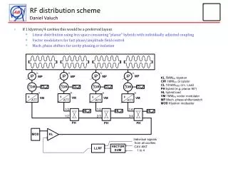
Klystron Cluster RF Distribution Scheme. Chris Adolphsen Chris Nantista SLAC. Baseline Tunnel Layout. Two 4-5 m diameter tunnels spaced by ~7 m. Accelerator Tunnel. Waveguides Cryomodules. Penetrations (every ~12 m). Service Tunnel. Modulators Klystrons Electrical Dist Cooling System.

E N D
Klystron Cluster RF Distribution Scheme Chris Adolphsen Chris Nantista SLAC
Baseline Tunnel Layout Two 4-5 m diameter tunnels spaced by ~7 m. Accelerator Tunnel Waveguides Cryomodules Penetrations (every ~12 m) Service Tunnel Modulators Klystrons Electrical Dist Cooling System
Klystron Cluster Concept Same as baseline RF power “piped” into accelerator tunnel every 2.5 km Service tunnel eliminated Electrical and cooling systems simplified Concerns: power handling, LLRF control coarseness
First Pass at New Tunnel Layout RF Waveguide
Waveguide Attenuation Assume smooth copper plated or aluminum walls: TE01: Transmission over 1 km for D = 0.480 m Cu: 0.9155 Al: 0.8932 Assume 48.0 cm Diameter between TE51 and TE22 cutoffs, 6.8% below TE02 cutoff (power)
Power Handling Scaling by pulse width dependence, we should try to keep surface fields below 10 MV/m in couplers. 40 MV/m (400 ns/1.6 ms)1/6 = ~10 MV/m pulse width ratio L-band design goal maximum X-band design goal maximum SLAC’s 5 cell L-band cavity runs stably with surface fields of 20 MV/m with 1 ms pulses - given the higher power of the ILC system, we are even more conservative by choosing a lower surface field limit (i.e. 10 MV/m). In the waveguide, 350 MW → ~1.9 MV/m peak, not on wall. We should be able to keep surface fields below 10 MV/m threshold while coupling in and out 10 MW increments.
Overmoded Bend (Two Approaches) TE20 Each TE01 bend is composed of two circular-to-rectangular mode converters and an overmoded rectangular waveguide bend. General Atomics high power 90° profiled curvature bend in 44.5 mm corrugated waveguide for TE01 mode at 11.424 GHz TE01 TE20 SLAC compact high power 90° bend in 40.6 mm circular waveguide tapered to overmoded rectangular waveguide for TE01 mode at 11.424 GHz
X-Band Launchers and Tapoffs from NLC/GLC Program Co-axial TE01 Fractional Tap-offs C. Nantista
ILC: Co-Axial Tap Off (CATO) About 1200 Required – Only Gap Length, Ridge Varies Wrap-Around Waveguide Gap 0.48 m Matching Ridge Coaxial Region Output Waveguide with Width Transition Design by Chris Nantista
Choice of Diameters mode cut-off diameters Dc (m inches) = TE01: 13.750” – Input/output diameter Largest commercial vacuum flange 18.898” (0.480 m) – Transmission pipe diameter Low loss and below TE02 cut off TE02: 25.175” – Step-up diameter (TE02 node at 13.750”) TE03:
Coaxial Power Division With gaps ranging from <3” to ~8½”, we can get the full range of couplings needed, from ~3% up to 50%. The various coupling designs will differ only in a) gap width and b) matching ridge. All couplers share a single common design for the wrap-around section. UNMATCHED Pc/(Pt+Pc) |H|m = 0.798 sqrt(P) = 14.7 kA/m @ 340 MW |E|m = 208 sqrt(P) = 3.84 MV/m @ 340 MW
Complete CATO RF Design |H|m = sqrt(P) |E|m = 208.3 sqrt(P) V/m pulsed heating: ~1.3 °C (Cu) ~2.7 °C (Al) S Matrix 14.7 kA/m @ 340 MW coupling: 6.86% (-11.64 dB) return loss & parasitic modes: < -56 dB 3.84 MV/m @ 340 MW
CATO Magnetic and Electric Fields WR650 5 MW big pipe step taper step taper big pipe |H| |E| weld weld vacuum flange vacuum flange Note different color scale used 5 MW vacuum window
First Launcher and Final Tap-off The scattering matrix for a lossless 3-port tap-off with coupling C and reference planes chosen to make all elements real (port 2→S22 real, port 1→S21 real, port 3→S31 real) can be written: tap-off 1 3 matched 2 Short port 1 at a distance l to reduce to a 2-port coupler and adjust C and l to achieve desired coupling. tap-off 1 3 (2’) l 2 (1’)
First combiner (launcher) and last tap-off (extractor) are 3 dB units reversed relative to the others and shorted (with proper phase length) at port 1. Power Combining: 2 2 2 2 2 … 1 1 1 1 1 3 3 3 3 3 -3 dB -3 dB -4.8 dB -6 dB -7 dB l Power Dividing: -3 dB -4.8 dB -3 dB 1 1 1 3 3 3 2 2 2 l
Concept Development Steps 5 MW 5 MW Step 1: Run 10 MW through back-to-back, blanked-off CATOs w/o pipe step up: no resonant rf build up 5 MW < 5 MW 350 MW Step 2: Add pipe step up, adjust shorts to resonantly produce 350 MW SW ~ 1 m
Step 3: Use resonant waveguide to build up the stored energy equivalent to 350 MW traveling waves - provides more realistic rf turn-off time if have a breakdown Resonant Line ~6.24 MW back-shorted tap-in 100 m of WC1890 -17.57 dB 350 MW Step 4: Use resonant ring to test bends and ‘final design’ tap-in/off Resonant Ring phase shifter ~6.24 MW directional coupler tap-off tap-in 200 m of WC1890 350 MW -17.57 dB
Required Power and Coupling(for a 100 m line or 200 m ring) Round trip loss:1.8 % Round trip delay time:823 ns (vs 800 - 9000 ns shutoff time in ILC) Stored energy:288 J Dissipated power:6.2 MW = input power to produce 350 MW critically coupled Critical coupling for the emitted field to cancel the reflected field =-17.5 dB. Tc=QL/w = 23.1 ms
Comparison to ILC • For ILC • Power in tunnel (P) = Po*(L – z)/L, where z is distance from first feed and L = distance from first to last feed • RF shut off time (t) = (zo + z)*2.25/c where zo is the distance from the cluster to first feed • Max of P*t/Po = 4.1 us for zo = 100 m, L = 1.25 km • Power 100 m resonant line or ring (t = 0.82 us) to begin study of breakdown damage • Would need 100 * 4.1/.82 = 500 m of pipe (two 250 m rings) and thee 10 MW klystrons to simulate maximum energy absorption (P*t) of ILC • But would be delivered at ~ twice the power in ~ half the time
LLRF Control • Use summed vectors from 32*26 cavities (instead of 26) to control common drive power to the klystrons. • The increased length adds ~ 9 us delay time to the response, so perturbations cannot be very fast (which should be the case as we will know the beam current before the rf pulse in the ILC). • Assumes uncorrelated, local energy errors are small • Do not see significant correlations in the cavity amplitude jitter in FLASH ACC 4-6 cavities. • If needed, could add 1 or 2 fast phase/amplitude controllers to each rf unit (to drive the unmatched cavities in the two 9-cavity cryomodules in the ACD scheme).
Fast Amplitude and Phase Control(AFT prototype for FNAL PD) Rated for 550 kW at 1.3 GHz and has a 30 us response time
Klystron Failure Available power scales as the square of the fraction of combined klystrons running. If one fails out of 35, only 33 klystrons worth of RF are delivered; the rest goes to various loads. The baseline is similar in that beam loading roughly doubles the gradient loss if one klystron is off – in this case however, one can detune the cavities to zero the beam loading if the klystron will be off for an extended period.
Scheme for Improved Reliability • Assume 34 klystrons are required to feed 32 RF units with sufficient overhead. • Combine 36 klystrons per cluster and operate with one off (cold spare) or, more efficiently, operate all at reduced voltage and 94.4% (34/36) nominal klystron power. • In the event of a klystron failure, turn on the cold spare or turn the voltage and drive up for the remaining 35 klystrons to 100%. For the cost of 5.9% added klystrons and related hardware and a cost of 2.9% discarded RF power when operating with one nonfunctioning klystron, we can maintain the availability of full power in the event of a single source failure per cluster. This won’t work if two or more fail in a given cluster combination, but that scenario should be rare.
Beam-to-RF Timing Relative beam (c) to rf (vg) travel times for each feed Upstream: 1.25 km (1/vg + 1/c) = 9.32 ms Downstream:1.25 km (1/vg - 1/c) = 0.98 ms For the upstream feed, the RF-to-beam timing will vary by 9.32 ms. Centered, this represents ± 0.8% of nominal fill time. To first order, the gradient variation this produces along the beam will probably cancel, but 1.25 km may be too long a distance for canceling this systematic error, leading to filamentation. As a remedy, the cavity QL’s and powers can be tweeked to vary the desired ti accordingly. This will be done anyway to deal the gradient spread.
Summary Surface klystron clusters can save ~ 300 M$ (~ 200 M$ from eliminating service tunnel and ~100 M$ from simpler power and cooling systems). The GDE Executive Committee encourages R&D to pursue this idea. The proposed CATO tap in/off design is likely to be robust breakdown-wise. Have a plan to demonstrate its performance, although with only 1/5 of the worst case ILC stored energy after shutoff. Need to better study: Waveguide fabrication and tolerances – too large to be drawn, but don’t want seams (KEK working with industry on this). Bend design – mode preserving; low-loss; support 350 MW, 1.6 ms; compact enough for tunnel Impact on LLRF control, energy spread minimization, & efficiency. Modifications to accelerator tunnel to accommodate waveguide plus other systems from tunnel systems.