Download
1 / 43
430 likes | 437 Views
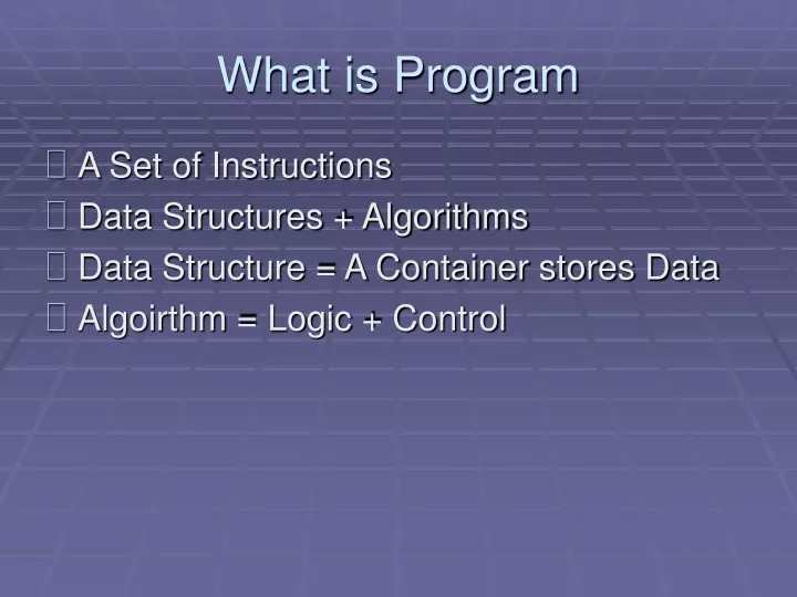
What is Program. A Set of Instructions Data Structures + Algorithms Data Structure = A Container stores Data Algoirthm = Logic + Control. Functions of Data Structures. Add Index Key Position Priority Get Change Delete. Common Data Structures. Array Stack Queue Linked List Tree

E N D
What is Program • A Set of Instructions • Data Structures + Algorithms • Data Structure = A Container stores Data • Algoirthm = Logic + Control
Functions of Data Structures • Add • Index • Key • Position • Priority • Get • Change • Delete
Common Data Structures • Array • Stack • Queue • Linked List • Tree • Heap • Hash Table • Priority Queue
Countless How many Algorithms?
Algorithm Strategies • Greedy • Divide and Conquer • Dynamic Programming • Exhaustive Search
Which Data Structure or Algorithm is better? • Must Meet Requirement • High Performance • Low RAM footprint • Easy to implement • Encapsulated
Chapter 1 Basic Concepts • Overview: System Life Cycle • Algorithm Specification • Data Abstraction • Performance Analysis • Performance Measurement
1.1 Overview: system life cycle (1/2) • Good programmers regard large-scale computer programs as systems that contain many complex interacting parts. • As systems, these programs undergo a development process called the system life cycle.
1.1 Overview (2/2) • We consider this cycle as consisting of five phases. • Requirements • Analysis: bottom-up vs. top-down • Design: data objects and operations • Refinement and Coding • Verification • Program Proving • Testing • Debugging
1.2 Algorithm Specification (1/10) • 1.2.1 Introduction • An algorithm is a finite set of instructions that accomplishes a particular task. • Criteria • input: zero or more quantities that are externally supplied • output: at least one quantity is produced • definiteness: clear and unambiguous • finiteness: terminate after a finite number of steps • effectiveness: instruction is basic enough to be carried out • A program does not have to satisfy thefinitenesscriteria.
1.2 Algorithm Specification (2/10) • Representation • A natural language, like English or Chinese. • A graphic, like flowcharts. • A computer language, like C. • Algorithms + Data structures = Programs [Niklus Wirth] • Sequential search vs. Binary search
1.2 Algorithm Specification (3/10) • Example 1.1 [Selection sort]: • From those integers that are currently unsorted, find the smallest and place it next in the sorted list. i [0] [1] [2] [3] [4] - 30 10 50 40 20 0 1030 50 40 20 1 10 2040 50 30 2 10 20 3040 50 3 10 20 30 4050
1.2 (4/10) • Program 1.3 contains a complete program which you may run on your computer
1.2 Algorithm Specification (5/10) • Example 1.2[Binary search]: [0] [1] [2] [3] [4] [5] [6] 8 14 26 30 43 50 52 left right middle list[middle] : searchnum0 6 3 30 < 434 6 5 50 > 434 4 4 43 == 430 6 3 30 > 180 2 1 14 < 182 2 2 26 > 182 1 - • Searching a sorted list while (there are more integers to check) { middle = (left + right) / 2; if (searchnum < list[middle]) right = middle - 1; else if (searchnum == list[middle]) return middle; else left = middle + 1; }
int binsearch(int list[], int searchnum, int left, int right) { /* search list[0] <= list[1] <= … <= list[n-1] for searchnum. Return its position if found. Otherwise return -1 */ int middle; while (left <= right) { middle = (left + right)/2; switch (COMPARE(list[middle], searchnum)) { case -1: left = middle + 1; break; case 0 : return middle; case 1 : right = middle – 1; } } return -1; } *Program 1.6: Searching an ordered list
1.2 Algorithm Specification (7/10) • 1.2.2 Recursive algorithms • Beginning programmer view a function as something that is invoked (called) by another function • It executes its code and then returns control to the calling function.
1.2 Algorithm Specification (8/10) • This perspective ignores the fact that functions can call themselves (direct recursion). • They may call other functions that invoke the calling function again (indirect recursion). • extremely powerful • frequently allow us to express an otherwise complex process in very clear term • We should express a recursive algorithm when the problem itself is defined recursively.
1.2 Algorithm Specification (9/10) • Example 1.3 [Binary search]:
1.2 (10/10) lv0 perm: i=0, n=2 abc lv0 SWAP: i=0, j=0 abc lv1 perm: i=1, n=2 abc lv1 SWAP: i=1, j=1 abc lv2 perm: i=2, n=2 abc print: abc lv1 SWAP: i=1, j=1 abc lv1 SWAP: i=1, j=2 abc lv2 perm: i=2, n=2 acb print: acb lv1 SWAP: i=1, j=2 acb lv0 SWAP: i=0, j=0 abc lv0 SWAP: i=0, j=1 abc lv1 perm: i=1, n=2 bac lv1 SWAP: i=1, j=1 bac lv2 perm: i=2, n=2 bac print: bac lv1 SWAP: i=1, j=1 bac lv1 SWAP: i=1, j=2 bac lv2 perm: i=2, n=2 bca print: bca lv1 SWAP: i=1, j=2 bca lv0 SWAP: i=0, j=1 bac lv0 SWAP: i=0, j=2 abc lv1 perm: i=1, n=2 cba lv1 SWAP: i=1, j=1 cba lv2 perm: i=2, n=2 cba print: cba lv1 SWAP: i=1, j=1 cba lv1 SWAP: i=1, j=2 cba lv2 perm: i=2, n=2 cab print: cab lv1 SWAP: i=1, j=2 cab lv0 SWAP: i=0, j=2 cba • Example 1.4 [Permutations]:
1.3 Data abstraction (1/4) • Data TypeA data type is a collection of objects and a set of operations that act on those objects. • For example, the data typeintconsists of the objects{0, +1, -1, +2, -2, …, INT_MAX, INT_MIN}and the operations+, -, *, /, and %. • The data types of C • The basic data types: char, int, float and double • The group data types: array and struct • The pointer data type • The user-defined types
1.3 Data abstraction (2/4) • Abstract Data Type • An abstract data type(ADT) is a data type that is organized in such a way that the specification of the objects and the operations on the objects is separated from the representation of the objects and the implementation of the operations. • We know what is does, but not necessarily how it will do it.
1.3 Data abstraction (3/4) • Specification vs. Implementation • An ADT is implementation independent • Operation specification • function name • the types of arguments • the type of the results • The functions of a data type can be classify into several categories: • creator / constructor • transformers • observers / reporters
1.3 Data abstraction (4/4) • Example 1.5 [Abstract data typeNatural_Number] ::= is defined as
1.4 Performance analysis (1/17) • Criteria • Is it correct? • Is it readable? • … • Performance Analysis (machine independent) • space complexity: storage requirement • time complexity: computing time • Performance Measurement (machine dependent)
1.4 Performance analysis (2/17) • 1.4.1 Space Complexity: S(P)=C+SP(I) • Fixed Space Requirements (C)Independent of the characteristics of the inputs and outputs • instruction space • space for simple variables, fixed-size structured variable, constants • Variable Space Requirements (SP(I))depend on the instance characteristic I • number, size, values of inputs and outputs associated with I • recursive stack space, formal parameters, local variables, return address
1.4 Performance analysis (3/17) • Examples: • Example 1.6: In program 1.9, Sabc(I)=0. • Example 1.7: In program 1.10, Ssum(I)=Ssum(n)=0. Recall: pass the address of the first element of the array & pass by value
1.4 Performance analysis (4/17) • Example 1.8: Program 1.11 is a recursive function for addition. Figure 1.1 shows the number of bytes required for one recursive call. Ssum(I)=Ssum(n)=6n
1.4 Performance analysis (5/17) • 1.4.2 Time Complexity: T(P)=C+TP(I) • The time, T(P), taken by a program, P, is the sum of its compile time C and its run (or execution) time, TP(I) • Fixed time requirements • Compile time (C), independent of instance characteristics • Variable time requirements • Run (execution) time TP • TP(n)=caADD(n)+csSUB(n)+clLDA(n)+cstSTA(n)
1.4 Performance analysis (6/17) • A program step is a syntactically or semantically meaningful program segment whose execution time is independent of the instance characteristics. • Example (Regard as the same unit machine independent) • abc = a + b + b * c + (a + b - c) / (a + b) + 4.0 • abc = a + b + c • Methods to compute the step count • Introduce variable count into programs • Tabular method • Determine the total number of steps contributed by each statement step perexecution frequency • add up the contribution of all statements
1.4 Performance analysis (7/17) • Iterative summing of a list of numbers • *Program 1.12: Program 1.10 with count statements (p.23)float sum(float list[ ], int n){ float tempsum = 0; count++; /* for assignment */ int i; for (i = 0; i < n; i++) {count++; /*for the for loop */ tempsum += list[i]; count++; /* for assignment */ }count++; /* last execution of for */count++; /* for return */ • return tempsum; } 2n + 3 steps
1.4 Performance analysis (8/17) • Tabular Method • *Figure 1.2: Step count table for Program 1.10 (p.26) Iterative function to sum a list of numbers steps/execution
1.4 Performance analysis (9/17) • Recursive summing of a list of numbers • *Program 1.14: Program 1.11 with count statements added (p.24)float rsum(float list[ ], int n){count++; /*for if conditional */ if (n) {count++; /* for return and rsum invocation*/ return rsum(list, n-1) + list[n-1]; }count++; return list[0];} 2n+2 steps
1.4 Performance analysis (10/17) • *Figure 1.3: Step count table for recursive summing function (p.27)
1.4 Performance analysis (11/17) • 1.4.3 Asymptotic notation (O, , ) • Complexity of c1n2+c2n and c3n • for sufficiently large of value, c3n is faster than c1n2+c2n • for small values of n, either could be faster • c1=1, c2=2, c3=100 --> c1n2+c2n c3n for n 98 • c1=1, c2=2, c3=1000 --> c1n2+c2n c3n for n 998 • break even point • no matter what the values of c1, c2, and c3, the n beyond which c3n is always faster than c1n2+c2n
1.4 Performance analysis (12/17) • Definition: [Big “oh’’] • f(n) = O(g(n)) iff there exist positive constants c and n0 such that f(n) cg(n) for all n, n n0. • Definition: [Omega] • f(n) = (g(n)) (read as “f of n is omega of g of n”) iff there exist positive constants c and n0 such that f(n) cg(n) for all n, n n0. • Definition: [Theta] • f(n) = (g(n)) (read as “f of n is theta of g of n”) iff there exist positive constants c1, c2, and n0 such that c1g(n) f(n) c2g(n) for all n, n n0.
1.4 Performance analysis (13/17) • Theorem 1.2: • If f(n) = amnm+…+a1n+a0, then f(n) = O(nm). • Theorem 1.3: • If f(n) = amnm+…+a1n+a0 and am > 0, then f(n) = (nm). • Theorem 1.4: • If f(n) = amnm+…+a1n+a0 and am > 0, then f(n) = (nm).
1.4 Performance analysis (14/17) • Examples • f(n) = 3n+2 • 3n + 2 <= 4n, for all n >= 2, 3n + 2 = (n)3n + 2 >= 3n, for all n >= 1, 3n + 2 = (n)3n <= 3n + 2 <= 4n, for all n >= 2, 3n + 2 = (n) • f(n) = 10n2+4n+2 • 10n2+4n+2 <= 11n2, for all n >= 5, 10n2+4n+2 = (n2)10n2+4n+2 >= n2, for all n >= 1, 10n2+4n+2 = (n2)n2 <= 10n2+4n+2 <= 11n2, for all n >= 5, 10n2+4n+2 = (n2) • 100n+6=O(n) /* 100n+6101n for n10 */ • 10n2+4n+2=O(n2) /* 10n2+4n+211n2 for n5 */ • 6*2n+n2=O(2n) /* 6*2n+n2 7*2n for n4 */
1.4 Performance analysis (15/17) • 1.4.4 Practical complexity • To get a feel for how the various functions grow with n, you are advised to study Figures 1.7 and 1.8 very closely.
1.4 Performance analysis (17/17) • Figure 1.9 gives the time needed by a 1 billion instructions per second computer to execute a program of complexity f(n) instructions.
1.5 Performance measurement (1/3) • Although performance analysis gives us a powerful tool for assessing an algorithm’s space and time complexity, at some point we also must consider how the algorithm executes on our machine. • This consideration moves us from the realm of analysis to that of measurement.
1.5 Performance measurement (2/3) • Example 1.22 [Worst case performance of the selection function]: • The tests were conducted on an IBM compatible PC with an 80386 cpu, an 80387 numeric coprocessor, and a turbo accelerator. We use Broland’s Turbo C compiler.