Download
1 / 22
220 likes | 339 Views
SPSS Session 1: Levels of Measurement and Frequency Distributions . Learning Objectives. Measurement of data Levels of measurement Measures of Central Tendency Measures of Dispersion. Review from Lecture 7. Identified and defined levels of measurement and measures of central tendency

E N D
SPSS Session 1:Levels of Measurement and Frequency Distributions
Learning Objectives • Measurement of data • Levels of measurement • Measures of Central Tendency • Measures of Dispersion
Review from Lecture 7 • Identified and defined levels of measurement and measures of central tendency • Described situations in which different levels of measurement and measures of central tendency were useful and appropriate • Calculated frequency, percentage, range, measures of central tendency • Critiqued and justified their use for the exercise problems
Levels of Measurement • The level of measurement used in collecting data determines the statistical techniques which can be used in analysis. • Levels of measurement: • Nominal • Ordinal • Interval/Ratio
Nominal Level Measurement • Classifying items into groups • No implied value of the groups as in a hierarchy or quantitative value • In the dataset from our child protection study, nominal variables include • Gender of the respondent and child • male or female • General Health Questionnaire elevated scores • Subclinical score or clinically elevated score
Ordinal Level Measurement • Classifying values of a variable in an order • Quantitatively ordered items with an implied qualitative order • An example is a Likert scale question with possible responses: • 1. Never, 2. Sometimes, 3. Occasionally, 4. Often, 5. Always • An example in our child protection study of an ordinal variable: • Previous_Involvement - Have Social Services been involved with this child/ family previously? • 1. Yes – Long standing involvement • 2. Yes – Occasional involvement • 3. No – No previous involvement
Interval/Ratio Level Measurement • Interval/Ratio level variables have equal units between variables and offer a range of possible values in that variable • Age, time, and weight are examples • Examples in our child protection study of interval/ratio variables are: • GHQ-12 total score • FES scores • WAI scores • Age of child • Other total scores from standardized measures
Frequency Distributions • A distribution provides a summary of how the data exists on a range of possible or actual scores. • A frequency distribution combines all of the like values of a variable and graphical groups them. • Which is to say how many times a value was recorded in a variable • Charts such as a histogram provide a visual display of a frequency distribution where the frequencies of similar values in a variable are grouped
Frequency Distributions • In our child protection study: • Gender of the child • Age of the child • Previous involvement with social services • Gender of the child is a nominal variable • Previous Involvement with social services is an ordinal variable • Age of the child is an interval/ratio variable • Use the Analyze Menu in SPSS to find “Frequencies”
Select the variables from the list on the left and place in the “Variable(s)” list on the right.
Click on “Statistics” and select “Mean”, “Median”, “Mode”, “Standard Deviation”, “Minimum”, and “Maximum” • Click “Continue”
Click on “Charts”, and select “Histograms” with “Show normal curve on histogram” • Click “Continue”
Frequency Distributions • Click “OK” for the Frequency Distributions and the descriptive statistics for these three variables. • The results will appear in a new Output window
In the first table, the descriptive statistics for the three variables are displayed.
Frequency Tables and Histograms • The next three slides give the Frequency Table and Histogram for each of the three variables we selected. • When comparing the tables to the histograms, look to see how similar values are combined and visually displayed in the chart. • Also, compare the distribution in the histogram to the curve of that the distribution would be if the variable were normally distributed.
Measures of Central Tendency • Mean – summing all the scores in a dataset and dividing by the total number of scores. Provides an average score. • Median – The middle most score in a list of scores • Mode – The most frequent or common score in a list of scores
Measures of Central Tendency • From these results, we can see that the mean of the children in the study was 7.69 years. • Remember that it is inappropriate to take means (averages) of nominal or ordinal variables, thus the Means and Std. Deviation scores for Child Gender and Previous Involvement should be ignored.