Download
1 / 23
290 likes | 877 Views
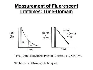
Measurement of Fluorescent Lifetimes: Time-Domain. Time-Correlated Single Photon Counting (TCSPC) vs. Stroboscopic (Boxcar) Techniques. Deconvolution. F(t) = i e -t/ I S(t) = L(t)F(t)dt. Time-Resolved Emission Spectra. Measurement of Fluorescent Lifetimes: Frequency-Domain.

E N D
Measurement of Fluorescent Lifetimes: Time-Domain Time-Correlated Single Photon Counting (TCSPC) vs. Stroboscopic (Boxcar) Techniques.
Deconvolution F(t) = ie-t/I S(t) = L(t)F(t)dt
Measurement of Fluorescent Lifetimes: Frequency-Domain Exciting Light:L(t) = a + bsin(t)( = 2 x freq.) Emitted Light: F(t) = A + Bsin(t - ) Lifetimes: tan = x p m = (B/A)/(b/a) = [1 + ²m²]-½
H N Fluorescent Molecules
H N Fluorescent Molecules • Intrinsic Fluorescent Probes (i.e. tryptophan): • Sensitive to local environment • Relatively small • Readily available in proteins • Generated by site-directed mutagenesis • Covalent Extrinsic Probes (i.e. TAMRA): • Broad range of spectral properties • Bright, relatively photostable • Well characterized conjugation chemistry • Non-covalent Probes (i.e. mant-ATP): • Similar properties to covalent probes • No need to permanently modify protein • Target active site or ligand binding sites
Protein Structural Dynamics: effects on fluorescence emission spectra Polarization experiments are sensitive to changes in orientation of a fluorescent probe. Spectral Shifts depend on the environment around a fluorescent probe. A more polar environment tends to red shift the emission spectrum and a less polar environment tends to blue shift the emission spectrum. Dynamic Quenching experiments are a quantitative way to measure the accessibility of a fluorescent probe to quenching molecules in the solvent. FRET (Fluorescence Resonance Energy Transfer) experiments can measure the distance between a donor probe and an acceptor probe on the protein.
Dynamic Quenching: measure accessibility to solvent and rates of diffusion. kq - bimolecular quenching constant, proportional to rate of diffusion of quencher or fluorophore. = kF/(kF + kNR) Q = kF/(kF + kNR + kq[Q]) kq[Q] = pseudo-first order rate constant (M-1s-1) since [Q] >> [F]. /Q = (kF + kNR + kq[Q])/ (kF + kNR) = 1 + kq[Q]/ (kF + kNR) and since = 1/(kF + kNR) /Q = 1 + kq[Q] Stern-Volmer Equation: F0/F = 1 + KD[Q] KD = kq = Stern-Volmer quenching constant. S1 kF kNR kq[Q] hv Plot of (F0/F - 1) vs. [Q] is linear with slope = KD. S0
Stern-Volmer Plots F0/F = = 1 + kq[Q] = 1 + KD[Q]
Static Quenching F0/F = 1 + KS[Q] Ks = equilibrium constant for quencher binding to fluorophore ([F-Q]/[F][Q]). Static quenching can be differentiated from dynamic quenching by: 1.) lifetime measurements - static quenching alters intensity, not lifetime. dynamic quenching alters both. 2.) temperature effects –
Combined Dynamic and Static Quenching: Stern-Volmer plot is concave upward. F0/F = (1 + KD[Q]) x (1 + KS[Q]) = 1 + (KD + KS)[Q] + KDKS[Q]2 =1 + Kapp[Q] therefore
Quenching Sphere of Action Therefore
Two Populations of Fluorophores: one accessible to solvent, one not. F = Fa + Fb = (F0a/(1 + Ka[Q])) + F0b (F0/(F0 – F)) = 1/(ƒK[Q]) +1/ƒ where ƒ = F0a/( F0a + F0a), a = accessible and b = buried.
1. Apoazurin Pf1 2. Ribnuclease T1 3. Staphylococcus nuclease 4. Glucagon
Collisional Quenching in Proteins Buried Residue Exposed Residue