Download
1 / 63
650 likes | 1.04k Views
Chapter 5: Process Scheduling . Chapter 5: Process Scheduling. Basic Concepts Scheduling Criteria Scheduling Algorithms Thread Scheduling Multiple-Processor Scheduling Operating Systems Examples Algorithm Evaluation. Objectives.

E N D
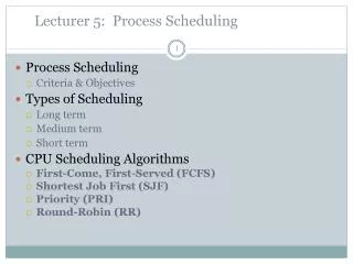
Chapter 5: Process Scheduling • Basic Concepts • Scheduling Criteria • Scheduling Algorithms • Thread Scheduling • Multiple-Processor Scheduling • Operating Systems Examples • Algorithm Evaluation
Objectives • To introduce process scheduling, which is the basis for multiprogrammed operating systems • To describe various process-scheduling algorithms • To discuss evaluation criteria for selecting a process-scheduling algorithm for a particular system
Basic Concepts • Maximum CPU utilization obtained with multiprogramming • CPU–I/O Burst Cycle – Process execution consists of a cycle of CPU execution and I/O wait • CPU burst distribution
Histogram of CPU-burst Times 155 2ms Alternating Sequence of CPU And I/O Bursts
CPU Scheduler • Selects from among the processes in memory that are ready to execute, and allocates the CPU to one of them • CPU scheduling decisions may take place when a process: 1. Switches from running to waiting state (I/O Request) 2. Switches from running to ready state (Timer timeout) 3. Switches from waiting to ready (I/O Completed) 4. Terminates • Scheduling under 1 and 4 is nonpreemptive • All other scheduling is preemptive
Dispatcher • Dispatcher module gives control of the CPU to the process selected by the short-term scheduler; this involves: • switching context • switching to user mode • jumping to the proper location in the user program to restart that program • Dispatch latency – time it takes for the dispatcher to stop one process and start another running
Scheduling Criteria • CPU utilization – keep the CPU as busy as possible • Throughput – # of processes that complete their execution per time unit • Turnaround time – amount of time to execute a particular process • Waiting time – amount of time a process has been waiting in the ready queue • Response time – amount of time it takes from when a request was submitted until the first response is produced, not output (for time-sharing environment)
Scheduling Algorithm Optimization Criteria • Max CPU utilization • Max throughput • Min turnaround time • Min waiting time • Min response time
P1 P2 P3 0 24 27 30 First-Come, First-Served (FCFS) Scheduling ProcessBurst Time P1 24 P2 3 P3 3 • Suppose that the processes arrive in the order: P1 , P2 , P3 The Gantt Chart for the schedule is: • Waiting time for P1 = 0; P2 = 24; P3 = 27 • Average waiting time: (0 + 24 + 27)/3 = 17
P2 P3 P1 0 3 6 30 P1 P2 P3 0 24 27 30 FCFS Scheduling (Cont) Suppose that the processes arrive in the order P2 , P3 , P1 • The Gantt chart for the schedule is: • Waiting time for P1 = 6;P2 = 0; P3 = 3 • Average waiting time: (6 + 0 + 3)/3 = 3 • Much better than previous case • Convoy effect:short process behind long process
Shortest-Job-First (SJF) Scheduling • Associate with each process the length of its next CPU burst. Use these lengths to schedule the process with the shortest time • SJF is optimal – gives minimum average waiting time for a given set of processes • The difficulty is knowing the length of the next CPU request
P3 P2 P4 P1 3 9 16 24 0 Example of SJF ProcessBurst Time P1 6 P2 8 P3 7 P4 3 • SJF scheduling chart • Average waiting time = (3 + 16 + 9 + 0) / 4 = 7
Determining Length of Next CPU Burst • Can only estimate the length • Can be done by using the length of previous CPU bursts, using exponential averaging
Examples of Exponential Averaging • =0 • n+1 = n • Recent history does not count • =1 • n+1 = tn • Only the actual last CPU burst counts • If we expand the formula, we get: n+1 = tn+(1 - ) tn-1+ … +(1 - )j tn-j+ … +(1 - )n +1 0 • Since both and (1 - ) are less than or equal to 1, each successive term has less weight than its predecessor
Prediction of the Length of the Next CPU Burst • (α = 1/2, τ0 =10)
Example of SJF Process Arrival TimeBurst Time P1 0 8 P2 1 4 P3 2 9 P4 3 5 • SJF scheduling chart • Average waiting time = ? P1 P1 P2 P3 P4 26 1 5 10 17 0
Priority Scheduling • A priority number (integer) is associated with each process • The CPU is allocated to the process with the highest priority (smallest integer highest priority) • Preemptive • Nonpreemptive • SJF is a priority scheduling where priority is the predicted next CPU burst time • Problem Starvation– low priority processes may never execute • Solution Aging– as time progresses increase the priority of the process
Round Robin (RR) • Each process gets a small unit of CPU time (time quantum), usually 10-100 milliseconds. • After this time has elapsed, the process is preempted and added to the end of the ready queue. • If there are n processes in the ready queue and the time quantum is q, then each process gets 1/nof the CPU time in chunks of at most q time units at once. No process waits more than (n-1)q time units. • Performance • q large FIFO • q small q must be large with respect to context switch, otherwise overhead is too high
P1 P2 P3 P1 P1 P1 P1 P1 0 10 14 18 22 26 30 4 7 Example of RR with Time Quantum = 4 ProcessBurst Time P1 24 P2 3 P3 3 • The Gantt chart is: • Typically, higher average turnaround than SJF, but better response
Turnaround Time Varies With The Time Quantum 5,3,1,5,1,2 = 15+8+9+17 = 49/4 = 12.25 6,3,1,6,1 = 6+9+10+17 = 42/4 = 10.5 6,3,1,7 = 6+9+10+17 = 42/4 = 10.5
Multilevel Queue • Ready queue is partitioned into separate queues:foreground (interactive)background (batch) • Each queue has its own scheduling algorithm • foreground – RR • background – FCFS • Scheduling must be done between the queues • Fixed priority scheduling; (i.e., serve all from foreground then from background). Possibility of starvation. • Time slice – each queue gets a certain amount of CPU time which it can schedule amongst its processes; i.e., 80% to foreground in RR, 20% to background in FCFS
Multilevel Feedback Queue • A process can move between the various queues; aging can be implemented this way • Multilevel-feedback-queue scheduler is defined by the following parameters: • number of queues • scheduling algorithms for each queue • method used to determine when to upgrade a process • method used to determine when to demote a process • method used to determine which queue a process will enter when that process needs service
Example of Multilevel Feedback Queue • Three queues: • Q0 – RR with time quantum 8 milliseconds • Q1 – RR time quantum 16 milliseconds • Q2 – FCFS • Scheduling • A new job enters queue Q0which is servedFCFS. When it gains CPU, job receives 8 milliseconds. If it does not finish in 8 milliseconds, job is moved to queue Q1. • At Q1 job is again served FCFS and receives 16 additional milliseconds. If it still does not complete, it is preempted and moved to queue Q2.
Thread Scheduling • User-level threads are managed by a thread library, and the kernel is unaware of them • To run on a CPU, user-level threads must ultimately be mapped to an associated kernel-level thread, although this mapping may be indirect and may use a LWP(Light Weight Process). • Contention Scope • process-contention scope (PCS) • system-contention scope (SCS) • One distinction between user-level and kernel-level threads lies in how they are scheduled.
Thread Scheduling • Many-to-one and many-to-many models, thread library schedules user-level threads to run on an available LWP (Light Weight Process) • Known as process-contention scope (PCS) since scheduling competition is among threads belonging to the same process • When we say the thread library schedules user threads onto available LWPs, we do not mean that the thread is actually running on a CPU; this would require the OS to schedule the kernel thread onto a physical CPU. • To decide which kernel thread to schedule onto a CPU, the kernel uses system-contention scope (SCS)
Thread Scheduling • Competition for the CPU with SCS scheduling takes place among all threads in the system. • System using the one-to-one model, schedule threads using only SCS. • Typically, PCS is done according to priority – the scheduler selects the runnable thread with the highest priority to run. User-level thread priorities are set by the programmer and are not adjusted by the thread library. • The PCS will typically preempt the thread currently running a favor of higher-priority thread; however there is no guarantee of time slicing among threads of equal priority.
Pthread Scheduling • API allows specifying either PCS or SCS during thread creation • PTHREAD SCOPE PROCESS schedules user-level threads using PCS scheduling • PTHREAD SCOPE SYSTEM schedules threads using SCS scheduling. • Will create and bind an LWP for each user-level thread on many-to-many systems, effectively mapping threads using the one-to-one policy.
Multiple-Processor Scheduling • CPU scheduling more complex when multiple CPUs are available • Homogeneous processors within a multiprocessor • Asymmetric multiprocessing (AMP)– • All scheduling decisions, I/O processing, and other system activities handled by only a single processor- the master server. • The other processors execute only codes. • Only one processor accesses the system data structures, reducing the need for data sharing
Multiple-Processor Scheduling • Symmetric multiprocessing (SMP) – • each processor is self-scheduling, • all processes in common ready queue, or • each has its own private queue of ready processes • Processor affinity – process has affinity for processor on which it is currently running • soft affinity – a process is possible to migrate between processors • hard affinity – a process is not to migrate to other processor
NUMA and CPU Scheduling • The main memory architecture can affect processor affinity issues. • An architecture featuring non-uniform memory access (NUMA) , in which a CPU has faster access to some parts of main memory than to other parts.
Multicore Processors • Recent trend to place multiple processor cores on same physical chip • Faster and consume less power • Memory stall – when a processor accesses memory, it spends a significant amount of time waiting for the data to become available.
Multicore Processors • Multiple threads per core also growing • Takes advantage of memory stall to make progress on another thread while memory retrieve happens Thread1 Thread0
Operating System Examples • Solaris scheduling • Windows XP scheduling • Linux scheduling
Solaris scheduling • Solaris uses priority-based thread scheduling where each thread belongs to one of six classes: • Time sharing (TS) • Interactive (IA) • Real time (RT) • System (SYS) • Fair share (FSS) • Fixed priority (FP) • Within each class there are different priorities and different scheduling algorithms. • Default class for a process is time sharing.
Solaris scheduling • The scheduling policy for the time-sharing class dynamically alters priorities and assigns time slices of different length using a multiple feedback queue. • There is an inverse relationship between priorities and time slices. • The following table shows dispatch table for time-sharing and interactive threads. • These two scheduling classes include 60 priority levels.
Solaris Dispatch Table Solaris dispatch table for time-sharing and interactive threads
Solaris scheduling • Priority: The class-dependent priority for the time-sharing and interactive classes. Ahigher number indicates a higher priority. • Time quantum: The time quantum for the associated priority. • Time quantum expired: The new priority of a thread that has used its entire quantum without blocking. Such threads are considered CPU-intensive and have their priorities lowered. • Return from sleep. The priority of a thread that is returning from sleeping (such as waiting for I/O). When I/O is available for a waiting thread, its priority is boosted between 50-59 – good response time for interactive processes.
Windows XP Scheduling • Windows XP schedules threads using a priority-based, preemptive scheduling algorithm. • Ensures the highest-priority thread will always run. • Dispatcher: The portion of the Windows XP kernel that handles scheduling. • A thread selected to run will run until it is preempted by a higher-priority thread, until it terminates, until its time quantum ends, or until it calls a blocking system call.
Windows XP Scheduling • 32-level priority scheme. • Divided into two classes • Variable class: threads with priorities 1-15 • Real-time class, 16-31 • Priority 0 for memory management thread • Idle thread: If no ready thread is found, execute the idle thread.
Windows XP Scheduling • The Win32 API identifies several priority classes to which a process can belong: • REALTIME_PRIORITY_CLASS • HIGH_PRIORITY_CLASS • ABOVE_NORMAL_PRIORITY_CLASS • NORMAL_PRIORITY_CLASS • BELOW_NORMAL_PRIORITY_CLASS • IDLE_PRIORITY_CLASS • Priorities in all classes except the REALTIME_PRIORITY_CLASS are variable, the priority of a thread belonging to one of these classes can change.
Windows XP Scheduling • A thread within a given priority class also has a relative priority : • TIME_CRITICAL • HIGHEST • ABOVE_NORMAL • NORMAL • BELOW_NORMAL • LOWEST • IDLE
Windows XP Priorities Priority Classes
Windows XP Scheduling • Each thread has a base priority representing a value in the priority range for the class the thread belongs to. • The base priority is the value of the NORMAL relative priority for that class. • The base priorities: • REALTIME_PRIORITY_CLASS -- 24 • HIGH_PRIORITY_CLASS -- 13 • ABOVE_NORMAL_PRIORITY_CLASS -- 10 • NORMAL_PRIORITY_CLASS -- 8 • BELOW_NORMAL_PRIORITY_CLASS -- 6 • IDLE_PRIORITY_CLASS -- 4