Download
1 / 34
340 likes | 524 Views
From The Stacker to Visibilities. Gordon Hurford, Ed Schmahl, Richard Schwartz 18-April-2005 Revised by EJS 13-July-2005. What is the Stacker?.

E N D
From The Stacker to Visibilities Gordon Hurford, Ed Schmahl, Richard Schwartz 18-April-2005 Revised by EJS 13-July-2005
What is the Stacker? Current imaging algorithms based on time-binned event lists • Time bins must be very short (~1-100ms) to preserve modulation -- Few events per bin (statistics, display, Forward Fit issues) -- Large number of bins (long integrations impractical) • Stacker is a form of superimposed epoch analysis • Compresses data from an arbitrarily long interval into the equivalent of a 1-rotation integration • Almost no loss of imaging information
How does the Stacker help? • Makes long integrations feasible But… solar rotation ~ 10 arcsec/hour at disk center • Some improvement to image quality • Improved c2 • Improved Forward Fit performance • Helps with background and flare-variability issues • Improvements in imaging speed • fewer time bins to fit • reuse stacked data (future) • Opens the way to visibilities
How does the Stacker work? (1) • Pointing changes • Phases are not duplicated rotation-to-rotation Cannot just stack data with rotation period • Count rate in each time bin depends on: • Source geometry and location • Grid transmission and slit depth • The occurrencetime of the bin is not relevant. • Roll angle & phase (relative to map center) are relevant Substitute roll angle / phase bins for time bins
How does the Stacker work? (2) • Stacker associates each time bin with a roll / phase bin • Accumulates counts and live time in each phase bin • Calculates average grid transmission and modulation amplitude for each roll / phase bin • Converts populated roll/phase bins back to equivalent time bins Existing mapping algorithms can be used as is
Mapping Time Bins to Roll/Phase Bins Roll angle (deg) Phase (relative to map center)
One Rotation Roll angle (deg) PHASE (relative to map center)
Multiple Rotations Roll angle (deg) PHASE (relative to map center)
Roll and Phase Bins Roll angle (deg) PHASE (relative to map center)
Populated Roll / Phase Bins Subcollimators 1-9 23 July 2002 12-25 keV 80-second integration Counts ____________________ livetime*gridtran*modamp c 23 July
Profiles in Roll Bins Subcollimator 5 25 March 2002 12-25 keV 80-second integration Counts/phase bin c 23 July
Stacked Modulation Profile Grid 8 7680 time bins 288 roll / phase bins
Comparison of Unstacked vs Stacked PIXON Maps Unstacked Stacked
Using the Stacker (1) • Default is not to use the stacker • No advantage if integration time is < ~ 3 rotations • Invoke with switch, /use_phz_stacker • Number of phase bins • Reduces S/N if too small. • Default=12 (99% efficient) • Obj -> set, phz_n_phase_bins = nnn
Using the Stacker (2) • Number of roll bins • Reduces s/n near edge of FOV is too small • Minimum value is determined by (max source offset) / (angular pitch) • Default: Number of roll bins is calculated automatically assuming source offset = 60 arcsec or image_dim * pixel_size/2 • To set source offset explicitly, phz_n_roll_bins_control = 0 phz_radius = nnn (arcsec) • To define number of roll bins explicitly, phz_n_roll_bins_control = [n1,n2,,,,n9] or n • Should the number of roll bins be even or odd? Even = conservative choice.
Status of the Stacker • Basic capability is in SSW in the atest subdirectory • Not yet systematically tested with all algorithms/options But seems to work fine with Clean and Pixons • No known bugs • To be implemented: • Better handling of variable flux & background • Features to support saving / retrieving / combining stacked counts from different intervals • Correction for solar rotation
RHESSI Visibilities What they are Their properties How they are measured An example How they can be used Status of software
A visibility is the calibrated measurement of a single Fourier component of the source. • Measured spatial frequency (arcsec-1): • Magnitude determined by the angular pitch of the grid. • Azimuth determined by the grid orientation at the time of measurement. • The measured visibility is a complex number (e.g. 100*eif) • Has amplitude and phase OR ‘sine’ and cosine’ components (e.g. A cos f, A sin f ) What are Visibilities?
Properties of visibilities (1) • Represent an intermediate step between modulated light curves and images. • Represent an (almost) noise-free transformation of input imaging data, containing all the imaging info required for mapping • Fully calibrated. • No remaining instrument dependence (other than spatial frequencies)
Properties of visibilities (2) • Statistical errors are well-determined because visibilities are linear combinations of binned counts. • Redundancy provides indication of systematic errors. • Amplitudes for visibility azimuths differing by 180 deg should be same. • Phases for visibility azimuths differing by 180 deg should be equal and opposite. • 3rd harmonic visibilities from grid n should match fundamental visibility from grid n-2. • Redundancy is independent of source.
Visibilities depend linearly on both the data and the source. • => Visibilities of a multi-component source • = sum of visibilities of its components • Very helpful in directly interpreting visibilities • Facilitates a visibility forward-fit routine • => Visibility measurements can be linearly combined. • Can add or subtract energy bands • Can add or subtract data over time • Can weight data in energy and/or time. Properties of visibilities (3)
How are visibilities measured ? • Visibility observations correspond to the modulation amplitude and phase • Can be measured from light curves directly • Problem of data gaps • Statistical issues • Normalization and sampling issues • Most easily determined from stacked data
Stacker Output as the Starting Point for Measuring Visibilitiesly Subcollimator 5 Measure amplitude & phase in each of 24 roll bins
Subcollimators 1 2 3 4 5 6 7 8 9 Aug 20, 2002 12-25 keV Polar plots of amplitude vs roll angle
How can visibilities be used? (1) • IMAGING: • Provide a compact representation of input imaging data • Can provide starting point for imaging algorithms • Useful for iterative processing • Ease statistical and c2 issues • Background is automatically removed. • Can be used with any radio astronomy imaging package
How can visibilities be used? (2) • Can infer quantitative source properties without mapping. • Source diameter • Source ellipticity • Source position • Statistical errors can be well-determined. • Provides a very sensitive tool for refining grid calibration
Currently testing a fragile version of software to calculate, display and exploit visibilities • Available offline to venturesome volunteers • Many features to be implemented • Testing for compatibility with latest version of hsi_phz_stacker • Handling of missing visibilities • Better ‘shell’ routine for convenient execution • Testing with use of automatic calculation of time and roll bins • Convenient tools for exploiting visibilities • Improved grid calibration • Calculation and application of statistical errors • Testing with harmonics • Integration of visibility analysis routines Status of Visibility Software